Voxel Space Automata
by Alerk Amin
Table of Contents
Figures
INTRODUCTION
Throughout nature, there is a delicate balance between order and randomness. From mountains to
oceans to plants, the seemingly random shapes of objects are actually based on a extremely
ordered foundation. The driving force behind computer graphics is to create realistic scenes,
from the largest objects down to the smallest subtleties of the texture. Nowhere is this
more important than in scenes involving nature.
Just as people decorate their homes with plants, graphic scenes look better with touch of
nature in them. Whether the purpose is to add a splash of color, or prevent a corner from looking
empty, plants can enhance any scene, whether indoors or outdoors. But to truly add to the image,
the plant should look real. This means that the balance between order and randomness must be
found in the structure of the plant.
The purpose of my Masters Project in Computer Graphics is to automatically create realistic plants
for use in computer generated pictures. Using the methods outlined by Greene in [1],
along with some personal additions, realistic plants can be created and included in images.
GOALS
The goal of this project is to create a C module for Data Explorer 2.0 [2].
This module takes a number of parameters as input, including the size of the plant, as well as
parameters that adjust the shape of the plant. It returns as output a field, consisting of lines,
that make up the plant. Existing Data Explorer modules can then place the plant inside a scene
and render it.
Another goal of the project is to enhance the module by making it multithreaded for parallel machines.
Large plants with many branches can take lots of CPU time to create, so splitting up the work and
distributing it among a few processors can significantly reduce the time required to construct the
plants. The module uses PVM3 [3] to run on a network of workstations.
APPROACH
The approach described by Greene involves starting a with a large, empty, 3 dimensional voxel space.
Then, starting with one or more seeds, grow the plant by changing voxels from unoccupied
to occupied. The plant is created by repeating a basic process:
At each node, try to grow a short distance. Test a few directions, and pick the best one based
upon the amount of light and sky reaching the node, as wells as the distance from other occupied
voxels (to avoid collisions). At some random nodes, create a new branch, using the same process.
If a node hits the edge of the allocated space, the node stops growing.
Although this method works well, it is extremely time consuming. A great deal of effort is taken
in finding the best direction to grow, when a good direction will do. In addition, leaves
are extremely difficult to place on the branches, and Greene's paper doesn't address them at all.
Also, the plants become tiny blocks, and although they may look fine from a distance, a closer
view of the plant would look jagged.
Another concern is that part of my project involves making this run in parallel. Splitting up a 3-d region
among a group of processor is an extremely difficult task. The load should be balanced between
processor, which is difficult for plant, since most plants have more branches near the top. Also,
as the plants grow into other regions, a great deal of overhead will be wasted in
synchronizing the processors, and checking neighboring regions for collisions.
To combat these issues, I decided to take advantage of Data Explorer's ability to render line segments.
By constructing the plant as a field consisting of many line segments, the jagged edges are eliminated.
In addition, by keeping a list of the nodes that need to be grown, the work can easily be split
among processors. Each processor takes a node off the list, grows it by one iteration, possibly
branching as well. Then, it inserts the new node(s) onto the list, and repeats the process. This
will ensure a good load balance, with very little communication between processes. In addition,
leaves can be constructed with small polygons placed at the ends of line segments.
GROWTH MODULE DESIGN
The Growth module, written for DX 2.0, was written increments. First, a single stem was grown.
Then, additional features such as attractors and collision avoidance were added. This section
describes the features in the order they were added to the module, as well as the issues the
brought up, and how the issues were resolved. Every parameter described in this section is
an input to the Growth module, and can be set by the user.
Basic Stem Growth
The plant starts with a single stem, located at the origin (0, 0, 0), growing towards the positive
z axis. The stem is grown by first offsetting the direction of growth a tiny bit, then growing
a fixed distance GROWTH_SIZE (the default is 5, but this can be changed) in that direction. When the
stem hits the edge of the bounding box, the stem stops growing.
A small direction adjustment is made by first finding a random vector within a narrow cone. This is
achieved by first creating a vector (0 ,0, GROWTH_SIZE). The vector is rotated between 0 and
10 degrees about the y-axis, and then rotated between 0 and 360 degrees about the z-axis. This gives a
vector with length GROWTH_SIZE, almost parallel to the z-axis. The rotations required to
make the z-axis point in the previous direction of growth are determined, then applied to the offset
vector. The result is a vector that points at a small angle (less than 10 degrees) from the previous
direction. The plant is grown in this direction, and the process is repeated.
The result is a stem that is grown in almost the original direction, but contains the small bends that make it
look real.
Branches
In dealing with branches, I also kept in mind the parallelism I would be adding later. To satisfy both
of these problems, I added a queue of branches to be grown. The queue starts with a single node, the
seed. The program dequeues an entry, grows it using the Basic Stem Growth algorithm, and computes
a new node, which it then enqueues, and repeats the process. However, for each node, it computes a function
that is true BRANCH_PROBABILITY per cent of the time. If the function returns false, no branch
is created. However, if the function is true, it creates a branch. Using a similar algorithm to the
Basic Stem Growth, it computes a direction that is between 40 and 60 degrees from the original direction.
It then grows in this direction, and enqueues this new node. The queue can become fairly long, if many
branches are created, resulting in a long list of nodes to be grown.
Greene uses a parameter called branch_age_range, which contains the number of iterations
before a stem branchs, picked at random for each stem. However, the percentage approach allows finer
control over the overall number of branches in the plant. In addition, it provides a basis for multiple
branches at the same node, which is describe later.
This approach supports parallelism well, because each processor can grow the nodes independent of the
other processors. The queue and output field must be shared between the processors, but nothing else.
Each processor can simply take an element off the queue, process it, update the output field,
enqueue the new nodes, and repeat the process. The processing stage, where the direction of growth is
jittered and new branches may be grown, depends only on data contained at local processor.
The main problem with branching is that multiple branches can run into each other. Since intersecting
branches doesn't happen to real plants, steps to avoid this were taken. But intersection isn't the
only problem. If a group of branches all grow into the same area, the plant is dense in this area,
and sparse in other areas. This also makes the picture look bad, since plants usually fill the
available space rather evenly.
Greene solves these problems by testing a bunch of directions, and picking the best one. If a good
direction cannot be found, the stem is not grown. This has the effect of creating short branches in
the middle of plants that look bad. My approach is to try and spread out the branches, so there is
a smaller chance of them entering the same region. My solutions to both of the problems are branch
avoidance and attractors.
Branch Avoidance
If a new branch is created along a stem, the next branch shouldn't point in the same direction. This
is the basic premise of branch avoidance in my design. Each stem keeps track of the direction
of the previous branch. It the stem creates another branch, the branch will be at least 90 degrees
from the previous branch. This is accomplished by saving the degrees the new branch was rotated about
the z-axis in the Basic Stem Growth algorithm. Then, when a new branch is created, the new
z-axis rotation is some value within a 180 degrees arc centered in a direction opposite to the
previous rotation.
Attractors
An attractor is a single point, usually outside the bounding box, that the plant has a tendency to
grow towards. In nature, the sun is an attractor. Since the branches of a plant are attracted
towards the sun, they grow upwards, and therefore do not collide with the lower branches of the
plant. Without attractors, using all the algorithms given above results in a direction that is independent
of the location of the node. Attractors use the location of the point to choose a direction.
Two of the inputs to the Growth module are the attractor_location, a Point, and the
attractor_strength, a number between 0 and 1. Using all the algorithms above, the module
computes a direction growth_dir to grow a branch. But before it grows the branch, it adjusts the
direction based on the attractor. From the current location of the node, it computes a vector
attractor_dir of length
GROWTH_SIZE, pointing to the attractor. It then computes a new growth direction as
a linear combination of these two vectors:
(attractor_strength)*attactor_dir + (1 - attractor_strength)*growth_dir. It normalizes this
vector to length GROWTH_SIZE, and then grows it. Note that for a small attractor strength,
the the result vector points closer to growth_dir, while for a higher attractor strength, it points
towards attractor_dir.
Segmenting & Multiple Branches
Segmenting is a tricky technique that puts significantly more control of the plant's structure in the
hands of the user. Rather than setting a single branch probability for the entire plant, the user
can divide the plant into 3 parts, and set the probability for each part. With the addition of
multiple branches, plants such as clovers, which have a single stem that breaks off into 3 or 4
branches, can be created.
The three segments are called the trunk, which consists of the part of the plant near the
seed, the limbs, in the middle, and the twigs, which are at the end. The user can
specify the number iterations required
for each part, and thus divide the plant into 1, 2, or 3 segments.
For each segment, the user can define the maximum number of branches at each node and the branch probability.
The branch probability is the probability for a single branch. For example, if a node has maximum
number of branches = 2 and branch probability = 50%, there is a 25% chance of no branches, 50% chance
of one branch, and 25% chance of two branches.
In the hands of a skillful user, segmenting and multiple branches allows a extremely wide variety of plants
to be created. However, it can also be very dangerous. It is very easy to create an extremely large number
of branches, making the Growth module run very slowly.
Parallelism
Because each node grows independent of the other nodes in the tree, fine grain parallelism can be achieved.
With more than one processor, each processor can be working on a single node simultaneously, greatly
reducing the amout of time required to produce a plant.
The parallel version of the module uses PVM3 [3] for communication between processes.
When the module is executed, the process that interfaces with Data Explorer registers with PVM and becomes the
"master" node. It then spawns a user-specifiable number of "slave" processes. PVM distributes these processes
among the available machines.
The master process becomes a server for the other slave processes, which do the actual computation. The master
starts by broadcasting the basic tree information, such as branch probabilities, sizes, and attractor location, to
the slave processes. In addition, it initializes the queue to the first node.
Each slave process requests a node from the master. The master receives these requests,
and sends nodes from the queue back to the slave processes.
The slave processes use the node information, as wells as the basic tree information, and compute a set of
new nodes, including any new branches. It then sends this information back to the master. The master enqueues
the new nodes, adding them to the appropriate field, and the process repeats.
When all nodes have been processed, the master sends a "dummy" node to the slave processes, which are still
requesting nodes. When the slaves get this node, they exit. The master then outputs the plant.
To the user of the module, the only difference is the addition of an input for the number of processors.
This parameter is the number of slave processes that are started. The optimal number of slaves is
usually the number of machines specified in the PVM hostfile, though not always.
Due to the nature of the parallel algorithm, the slaves may get nodes in different orders on different executions
of the module. Therefore, running the module twice with the same inputs will usually result in different outputs.
To make a sequence of images with the same plant, it is better to use the serial version.
RESULTS
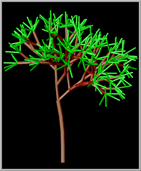
Figure 1. A basic tree
This basic tree shows many of the feature of the Growth module. The trunk segment is the thick line at the
bottom. No branches are allowed for this portion. The limbs segment allows branching, and usew a smaller
radius for the tube module. The twig segment is rendered in green, and has a depth of 1. It also has a very
high number of branches, and a high branch probability, to give the bursts of green at the ends of the limbs.

Figure 2. A fern
This fern is created by having a very small trunk and limb depth, with many branches. Then, the twigs are
given a large depth, but no branches. By placing the attractor below the origin, the plant grows downward.
This makes the long, hanging vines that distinguish ferns. All the fields are colored green, with small
tube radii.

Figure 3. A palm tree
This palm tree exemplifies segmenting. The trunk is made rather long, with no branches. Then, the limbs
are given a depth of one, with a high number of branches. This causes the burse of limbs at the end
of the trunk. Then, the twigs are given large depths, with no branches. Once again, the attractor is
placed below the origin, causing the twigs to bend downward. The trunk is made thick and brown, while
the limbs and twigs are thin and green.

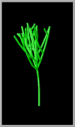
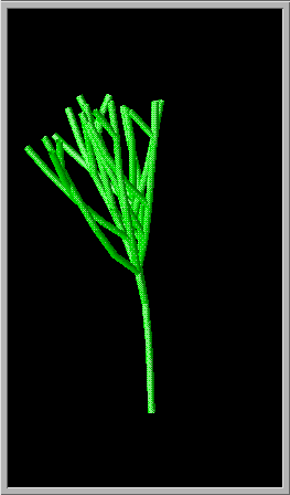 Figure 4. A sequence of images with a moving attractor
This sequence shows the benefit of the attractor. In the first image, the attractor is to the right of the plant. In the
second image, it is directly above the plant. In the third image, it is to the left of the plant. The result is the
plant "follows" the attractor. By creating many more frames, it is easy to construct a movie of a plant following
the sun across the sky.
GETTING THE MODULES
For both versions of the modules, it will be necessary to edit the Makefiles to reflect the locations of
libraries on your system. Makefile, queue.c, queue.h, and user.mdf are different between the two
versions. Be sure to get the right one.
Serial Version
The required files for the Serial Version are:
Parallel Version
The required files for the Parallel Version are:
USING THE MODULES & EXAMPLES
The main point to keep in mind is that it is easy to create thousands and thousands of branches, which
will take most computer a very long time to computer. For each segment, the number of nodes at the
end of the segment is approximately
(1 + max_number_of_branches * branch_probability)^depth
So the number of nodes at the tip of the tree is
number_of_nodes(trunk) * number_of_nodes(limbs) * number_of_nodes(twigs)
And the interior of the tree is even more nodes.
Each input of the Growth modules is either an integer or a float. The only difference between the Serial
and Parallel version is the Parallel has an extra parameter for the number of slave processes. The three
outputs correspond to the trunk, limb, and twig segments. To make them into a single field, use the
Group module. See the user.mdf files for more information on inputs and outputs.
For each of these examples, there are control panels to easily change the attractor strength and location,
the parameters for each segment, and the random seed. Use the "Open Control Panels" menu option in DX to
get access to these.
Serial Examples
The serial examples all correspond to the images shown in the results section of this document.
Parallel Examples
Because the parallel version can produce different results for the same input, based on the order the slaves receive
nodes, no sample picture is given. The example uses 2 slave processes, and there is no control panel to change the
number of slaves, but it can be added.
CONCLUSIONS & FUTURE WORK
The Growth modules are an attempt to create realistic plants and trees, using some simple algorithms. There are a number
of options that could be added to give the user more control over the look of the plants.
One option that could be added to both the Serial and Parallel versions is having different attractors for each segment.
This would allow the palm tree's trunk to be attracted upwards, and the twigs downwards. Another option is having
branches be their own segment, rather than having segments based on depth. This would allow for a thick trunk segment
all the way to the top of the tree, then have thinner limbs off the trunk, and even thinner twigs off the limbs.
A feature that could be added to the parallel version are syncronizing on the random number generator, to make the
parallel version produce the same tree with the same inputs. Another addition would be to allow slaves to grow
more than just one iteration, to reduce communication. The load could still be balanced well if slaves grew out
an entire segment, rather than just one iteration.
Of course, leaves can be added to make the plants look much better. The procedure to calculate a direction
of growth for leaves has already be implemented, and it remains to just add the leaf polygons to the
field. More than any other feature, leaves would make the plants more real.
The Growth module can serve as a basis for a great deal of future work in other types of growth, such as
crystal growth. With some more additions, the module can become faster and produce better plants. But as
it stands, plants can easily be included in Data Explorer images.
References
[1] Greene, Ned "Voxel Space Automata: Modeling With Stochastic Growth Processes
In Voxel Space" Computer Graphics, July 1989. pp. 175-184
[2] IBM Data Explorer 2.0. For more information, click
here
[3] Parallel Virtual Machine 3.0, Oak Ridge National Laboratory. To get PVM,
send email to netlib@ornl.gov with the message: send index from pvm3. You will receive
a list of available files and further instructions.


 Figure 4. A sequence of images with a moving attractor