Kriging Interpolation

by Chao-yi Lang, Dept. of Computer Science, Cornell University

Introduction
Goal
Theory
Implementation
Programs
Result
Conclusion
Acknowledge
References

Figures

An example of exponential variogram model
Estimated values
Error variance

INTRODUCTION

In real world, it is impossible to get exhaustive values of data at every desired point because of pratical constraints. Thus, interpolation is important and fundamental to graphing, analysing and understanding of 2D data.

The word "kriging" is synonymous with "optimal prediction"[1]. It is a method of interpolation which predicts unknown values from data observed at known locations. This method uses variogram to express the spatial variation , and it minimizes the error of predicted values which are estimated by spatial distribution of the predicted values.

GOAL

The goal of this project is to implement an ordinary kriging module for IBM Data Explorer 2.0 using C language. This module takes a number of input data, including a field of observed data, the estimated range, the resolution of the estimated range, variogram model, nugget effect and sill. The output is a field of estimated value and error variance.

THEORY

In ordinary kriging, which estimates the unknown value using a weighted linear combinations of the available sample[2]:

(1)

The error of i-th estimate, ri, is the difference of estimated value and true value at that same location:

(2)

The average error of a set of k estimates is:

(3)

The error variance is:

(4)

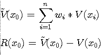
Unfortunately, we can not use the equation because we do not know the true value V1,...,Vk. In order to solve this problem, we apply a stationary random function that consists of several random variables, V(Xi). Xi is the location of observed data for i > 0 and i <= n. ( n is the total number of observed data). The unknown value at the location X0 we are trying to estimate is V(X0). The estimated value represented by random function is:

(5)

The error variance is :

(6)

is the covariance of the random variable V(X0) with itself and we assume that all of our random variables have the same variance.

is the Lagrange parameter[2].

In order to get the minimum variance of error, we calculate the partial first derivatives of the equation (6) for each w and setting the result to 0. Here is the example of differentiation with respect to w1:

(7)

All of weight Wi can be represented as:

For each i, 1 <= i <= n (8)

We can get the each weight Wi through the equation (8). After getting the value, we can estimate the value located in X0.

IMPLEMENTATION

The project uses variogram instead of covariance to calculate each weight of equation (8). The variogram is :

(9)

The minimized estimation variance is:

(10)

The kriging module includes two variogram models:

1. spherical

2. exponential

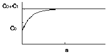
Nugget effect (c0) :

Though the value of the variogram for h = 0 is strictly 0, several factors, such as sampling error and short scale variability, may cause sample values separated by extremely small distances to be quite dissimilar. This causes a discontinuity at the origin of the variogram. The vertical jump from the value of 0 at the origin to the value of the variogram at extremely small separation distances is called the nugget effect.[2]

Range (a) :

The distance of two pairs increase, the variogram of those two pairs also increase. Eventually, the increase of the distance can not cause the variogram increase. The distance which cause the variogram reach plateau is called range.[ Figure 1]

Sill (C0 + C1) :

The maximum variogram value which is the plateau of Figure 1.

Distance h :

The distance between estimated location and observed location.

Figure 1. An example of an exponential variogram model

The equation (8) can be written in matrix notation as

V * W = D

V: is (n+1)X(n+1) matrix which contains the variogram of each known data. The components of last column and row are 1 and the last component of the matrix is 0.

W: is (n+1) matrix which contains the weight corresponding to each location. the last of component of matrix is Lagrange Parameter.

D: is (n+1) matrix which contains the variogram of known data and estimated data. The last component of the matrix is 1.

Since V and D is known, we can get the unknown matrix W by :

W = invert(V) * D

Applying equation (5), we can get the estimated value on a specific location. We also can get the error variance from the square root of equation(10).

PROGRAMS

The kriging module was implemented in two machines, IBM RS/6000 and HP-700. It is necessary to put the right library directory in the makefile. Some of the source codes were from netlib. Those source codes are used to invert matrix and were implemented by FORTRAN language originally. The FORTRAN codes have been translated to C code using the tool "f2c". The C code to invert the matrix is also need some special head file and library during compiling if your machine has no such library and head file.

inv_m.tar.gz The inverse matrix source codes which got from Netlib.

f2c.tar.gz The head file and library which are used to inverse matrix source codes.

krig.net The example dx file.

data1.dx The input example.

RESULT

There are 46 observed samples in input file. The range of estimate is minimum and maximum values for X and Y coordinate of observed sample locations. The output including estimated values (Figure 2.) and error variance (Figure 3.).

Figure 2. Estimated values

Figure 3. Error variance

Figure 2 shows the estimated area using the sample data. Figure 3 uses a colormap to display error variance. The red color area represents that the variance values are larger than other color areas. The blue color area represents that the variance values are less than other color areas. It is very clear to find that the error variance is small if there exists observed data. The location of white point represent the location of input data and the size of the white point means the elevation of the observed data.

CONCLUSION

Many properties of the earth's surface vary in an apparently random yet spatially correlated fashion. Using kriging for interpolation enables us to estimate the confidence in any interpolated value in a way better than the earlier methods do.[3]

Kriging is also the method that is associated with the acronym B.L.U.E. ( best linear unbiased estimator.) It is "linear" since the estimated values are weighted linear combinations of the available data. It is "unbiased" because the mean of error is 0. It is "best" since it aims at minimizing the variance of the errors. The difference of kriging and other linear estimation method is its aim of minimizing the error variance.

The project is to build a ordinary kriging module for IBM DataExplorer 2.0 using C language. Before using this module, it is important to know the meaning of input parameters and how to use it because those inputs values can not calculate from input sample data.

REFERENCES

[1] A. G. Journel and CH. J. Huijbregts " Mining Geostatistics", Academic Press 1981