
My goal for this independent research was to find out as much as I could, in 2 credits' time, about emergent processes in computer modeling and bottom-up computation. Both refer to a type of computation in which the final behavior of a program, or system, is not thoroughly specified by the prgrammer. Rather, the final behavior depends on a (often small) set of simple interactions which are specified, and usually have little to do with the desired overall behavior. When objects interact as specified, the resultant behavior is usually much more complex and interesting than the specified interactive behavior.
'Emergent processes' refers to complex behavior that arises when a very many instances of a certain object interact in often simple ways. A good example of this is the classical motion of the planets (ignoring the negligible forces other than gravity). Even though each particle in the Solar system obeys a simple gravitational law (the gravitational force between any two objects is proportional to both their masses and inversly proportional to the square of the distance between them) the result of all those interactions leads to the orbiting behavior of planets and moons, which is in no way encoded in the interaction between any two particles. That is to say, no interaction has the 'intent' of producing the outcome we percieve, yet that behavior emerges from the system. Other good examples of bottom-up processes include schooling of fish; flocking of birds; fluctuation in economies. Craig Reynolds has an excellent page on "Boids", his exploration in bottom up processes in the form of flocking birds.
The emergent process I implemented is self reproduction in patterns on a grid. Many people are familiar with Conway's game of Life, which isn't really a game but rather a simple model of emergent processes. This model consists of a regular grid of square cells, each of which is either 'alive' or 'dead'. Each cell can have either state in any one 'generation', that is, state of the grid as a whole. In any generation, the 'alive' or 'dead' property of each cell depends on how many of its eight grid-neighbors were alive or dead in the previous generation. When this grid is viewed graphically with 'alive' and 'dead' as separate colors, interesting, regular, and often beautiful patterns arise. The individual cells of the grid are often referred to as cellular automata. See this page for a good running example of the game of Life.
Christopher Langton (editor of Artificial Life, Proceedings in a Conference) described a grid of cellular automata whose states and prespecified rules permitted the existence of a pattern which reproduces itself in a neighboring area of the grid. The states of cells in this grid, instead of being 'alive' or 'dead', are numbered 0 - 7, and are visualized as colors. Here is what the first 'seed' generation looks like:

I used Microsoft Foundation Class to do the windowing and the execution of computation, which had to be performed in a separate thread to be free of windows-messages dependence. It was quite a chore going through MFC. You can download the executable, code, and MSDev workspace to check it out.
The second topic I set out to explore is bottom-up processes. In this type of computation, the programmer sets out to solve a problem using a method that does not attempt to embody what the programmer feels he/she knows about the problem in order to solve it, but rather, through the interaction of prespecified purely local processes. The problem I chose is the recognition of handwritten digits, and the bottom up process I chose is a neural network. It would be difficult to enter an introductory discusstion of neural networks; I would refer the interested to Judith Dayhoff's book, Neural Network Architectures, an Introduction. In addition, I attempted to use a genetic algorithm in conjuction with the neural network. Genetic algorithms concern themselves with optimizing the value of certain parameters, through a competitive search through parameter-space, when an exhaustive search is impossible because of the size of the space. An implementation of a genetic algorithm would instantiate several candidate "solutions," or points on the parameter-space. I will refer to these instances (rather standartly) as "individuals." The parameters can be referred to as "genotypes," completely describing the individual as far as the implementation is concerned. Each individual in the population is assigned a certain fitness, which corresponds to how well the parameters embodied by the individual's genotype optimize the desired value. The performance of the parameters encoded in the genotype can be thought of as the individual's phenotype. After all individuals' (all members of the "population") fitness is examined, some individuals are selected, and others are not (according to a prescribed scheme), parallelling natural selection in evolution theory. Using the selected individuals, a new generation of individuals (a new population) is created, again using one of a variety of schemes. Some individuals may have their phenotype mutated. Then the cycle begins again, with evaluating fitnesses, and continues until an individual with appropriate fitness is found. The parameters embodied in that individual's genotype are considered a solution to the posed optimization problem. For a more thorough introduction to genetic algorithms, see Melanie Mitchell's book, Introduction to Genetic Algorithms.
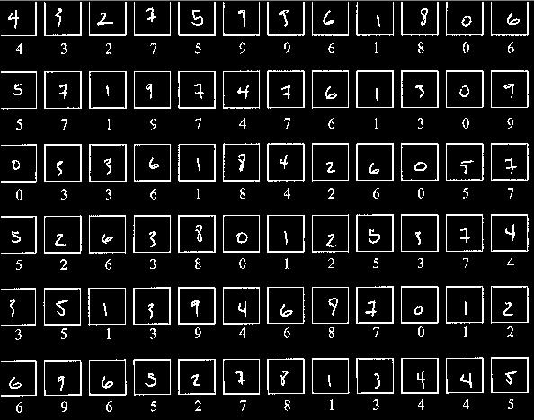
The neural network I implemented (at first, without a genetic algorithm) uses digitized images of handwritten digits as input. The collection of this data was rather laborious and included a totally separate program I had to write to assist me in the task. Since I could not find a resource of such data, I went around campus asking various people to fill in a sheet of paper with digits. The following is the top half of such a sheet: (the colors are reversed)


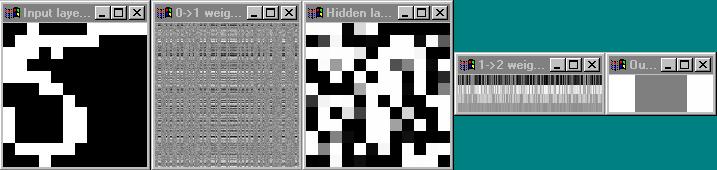
The windows, from left to right, visualize: the input layer; the weights between the input and the hidden layer; the hidden layer; the weights between the hidden layer and the output layer; the output layer.
Unfortunately, I could not get the neural net to train properly. It would always converge very early (after 2-3 training examples) on a set of weights which was obviously wrong. I suspect that the failure to train is due to the values I chose for some of the parameters for back-propagation, including the learning rate, momentum, and temperature. All interact in a non-linear way, and I had no precedent to establish good values for those parameters.
I had hoped that a genetic algorithm would alleviate that problem, in that it does not rely on back-propagation (or its associated parameters), but rather treats the weights between the layers as genotypes, the parameters to be optimized. I wrote code that would instantiate a population of 50 individuals (50 neural nets) whose weights are initially random. Each is evaluated a number of times (the net is run to produce output) to determine its fitness. Then individuals are ranked according to fitness (using quicksort) and chosen to be a 'parent' to the next generation with a probability corresponding to rank. Some low-ranked individuals are always selected to increase diversity, a known way to speed divergence in a genetic algorithm. Then, for each member of the new generation (the population is fixed in size) parents are paired at random, and two-point crossover is implemented. Crossover is the means by which a descendent individual combines the genotypes of both parents. Two-point crossover chooses two points in the genotype (considered linearly); the descendant acquires the parameters of the first parent that come before the first crossover point, the parameters of the second parent between the first and second points, and the parameters of the first parent after the second crossover point. This ensures that individual parameters residing near the ends of the genotype (considered linearly) do not always travel together, that is, they are just as likely to be crossed over as parameters residing in any other location. Two-point crossover is implemented twice for each descendant individual, once for the weights between the first and second layer, and once between the weights between the second and output layer. Unfortunately, I did not have enough time to finish the code, and although I believe it to be complete, it does not compile as it now stands.
You can get all the code, sample data, and MSDev workspace info.
Or maybe you prefer to just get my data. The only comparable thing I've seen would have cost me over $900 over the internet, so you lucked out! At least mail me so I can know my data is useful.