(ColorXY (cos u) (sin (+ u (sin (% (cos u) (sin (/ (tan t) (cos (log (sin (/ t t)) (log u (hsin t)))))))))) (log (tan -2) t)
Over the course of this semester, we have investigated the use of computers to solve problems through evolutionary means. We started by considering two distinct types of problems. First, we considered how to get a computer to learn to draw some object, like a human face. We wanted to design a system which would allow a computer to begin drawing a random object and learn to draw a face or a nice color pattern. The latter is similar ot the work done by Karl Sims [1]. It would make small modifications to its initial drawing and through user feedback, it would learn which modifications were good and which were bad. By repeating this process, the computer would eventually draw objects that resemble faces. The second problem we considered was the mathematical problem of fitting a curve to a set of points. In this case, the computer would be given a set of points and would then generate a random curve. It would check how close to the points the curve is and then make some modifications. By repeating the process, the computer would ultimately find a curve that contains all of the points. The advantage to this problem is that the computer determines for itself what is a good change rather than having a user tell it. This speeds up the process greatly which is important since many modifications on the initial data will generally be required. Thus, the two general types of problems we considered are those which the computer can judge for itself how it is doing and those which require human feedback.
The kinds of problems we considered all can be solved by evolutionary means. In this section, we explain precisley what an evolutionary algorithm is, highlight some of the theory behind evolutionary algorithms, and define important terms.
The idea behind evolutionary programming is the same as that behind natural evolution - survival of the fittest. We start off with a large number of random programs and evolve them. Some programs will not be fit (i.e. their execution generates poor results, as defined by the programmer) and will die off. Others will be fit and will survive into the next generation as well as produce children programs that inherit much of their parents' code. The children are produced in two ways: mutation and crossover. Mutation requires one parent program which is randomly mutated to create a child program. Crossover requires two parents which swap parts to produce two new children. Hopefully, after many generations the population of programs will include highly fit individuals that solve the particular problem.
There are many issues associated with successfully evolving programs. The language that the programs are written in has to be well-suited for the particular problem being solved. Programs in this language have to have some structure that allows for easy evolution of programs. At the same time the language has to include enough operators to create programs that can reasonably be expected to solve the given problem. The number of programs in each generation has to be large for a sufficient diversity in the genetic pool (but not too large, otherwise the process of evolution takes too long). There must be a way of determining how fit a given program is - this could be done automatically or it might require a person. Finally, there are many decisions to be made about how evolution is to proceed - how big the initial random programs are, how many children are generated by mutation and how many by crossover, how "severe" can a mutation or a crossover be (how much the children will differ from their parents), how many of the fittest programs survive into the next generation, whether any of the unfit programs might survive, how many children can unfit programs generate, etc.
Here are definitions of the key terms:
Fitness - how well a program solves the problem it is designed to solve
Selection - the means of deciding the fitness of a program
Generation - one time step in the evolution
Population - the set of programs in one generation
Crossover - creating children programs by splicing parts of one parent program into another
Mutation - creating children programs by randomly modifying parts of a single parent's program
Survival - when a program is carried over from the previous generation into the current generation
We implemented a graphical system to solve problems through evolution called EGO (Evolutionary Graphics Observer). There are three main parts to EGO. It is an interpreter of a graphical programming language, a simple graphics renderer for the language, and a system for evolving programs in the language through random mutations and crossovers.
One important aspect of the graphical language we created was that programs could be modified easily without causing the program to stop working. We therefore decided that a language in the style of LISP was the best choice. We could then substitute almost any expression with any other expression and the program would still make sense. A LISP-like language can easily be parsed into many expressions and subexpressions, making random modification easy. Any expression or subexpression can be replaced by any other expression or subexpression without having to consider how the expression fits into the rest of the program. The language we created, GOLLL (Graphically Oriented LISP Like Language) is outlined here.
EGO includes GOLLLI, an interpreter for the language. GOLLLI can read and parse a GOLLL program from a text file, write a GOLLL program to a text file, and evaluate the LISP-like expressions that make up the core of a GOLLL program. The C code for GOLLLI is included here. A GOLLL program is stored in a Program structure that keeps track of the number of variables in the program (defined by DefVarList and DefVarRange), number of DrawXY statements, and number of ColorXY statements (0 or 1). It also contains pointers to linked lists VariableList and DrawXYList and pointer to ColorXY structure. Every expression (X and Y components of DrawXY and R, G, B components of ColorXY) is stored in Expression structure and each operand in an Expression is stored in Operand structure. Every operand can be either a constant, a variable, or another expression.
The renderer of GOLLL programs involves simple scaling and display of points to fit in a window of a given size. Brief implementations details are provided now. The user can specify the size of the graphics window they desire. Then, an array of size x*y of RGB values is stored for any image to be drawn in the graphics window (assuming x and y are the width and height of the window, respectively). The RGB values are stored as COLORREF values, a Win32 way of expressing the red, blue, and green values. There are two main kinds of images that can be displayed: color patterns and parametric curves of one variable. To display parametric curves, a linked list of points is passed in. The mean x and y values are calculated as well as the standard deviation from the mean. These are used to give the graphics window a scale which centers the points in the graphics window and removes any outliers. Once the window has some scale, the points can be added to the image array with a color of black (the image array defaults to a white background). To display color patterns, a similar process is followed, but the points passed in must have integral x and y values in the range zero to the width and height of the window. Each point comes with a color value. In this case, the color values must be scaled to between 0 and 255. This is done by calculating each color value mod 256. Then, the colors are scaled so that the highest value is 255. The code for displaying these two kinds of patterns can be found here.
The evolving system evaluates the fitness of the programs in each generation, then creates a new generation of programs. It is also responsible for creating the original population. The are a large number of parameters that can be set by the user that control the process of evolution. For the original population the user specifies the proportion of variables to constants, the proportion of trig functions (sin,cos,tan) to exponential functions (c^n, log) to arithmetic functions (+,-,*,/), the average size of a program, and whether to create color patterns, parametric curves, or both. For creating a subsequent generation, the user can specify the proportion of survivors to mutants to crossovers and the proportion of parents with high fitness to parents with low fitness (low fitness parents can be important for getting the system to stop converging on a solution that is not optimal). For mutations, the user can specify probabilities of going between constants, variables, and expressions as well as the number of mutations to do in each step. For crossovers, the user can specify the number of crossovers to do and how many subexpressions the part being swapped should contain. The latter two groups of parameters are used to modify the Expression structures of programs to create new working programs. The code for mutations, crossovers, random program generation, and evolution can be found here.
The executable for our system (about 1MB size) (which runs on Windows NT 4.0) is here.
The user's guide for the EGO application is here.
Generating Color Patterns
We achieved good results generating random color patterns and watching them evolve. We could manually set the fitness of each color pattern (that is, we ranked each image in order of how we like it).
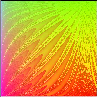
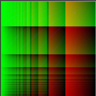
The following images came from 15 generations created in this manner. The first two images show a clear example of one program mutating into another program. Notice the streaks running down the image in the second one that are not present in the first. This is due to a crossover with another image. Also note the increasing program size between the earlier and the later generation. This is due to mutations of variables and constants into complex expressions as well as crossovers.
Many of the patterns we generated were comparable in complexity and even sometimes in structure to the ones generated by Karl Sims [1]. But it seems unlikely that our system matches Sims' system's potential for generating various patterns. The reason for that is the large number of operators that Sims's system had and our does not (noise, warps, color-grad, blur).
(ColorXY (cos u) (sin (+ u (sin (% (cos u) (sin (/ (tan t) (cos (log (sin (/ t t)) (log u (hsin t)))))))))) (log (tan -2) t)
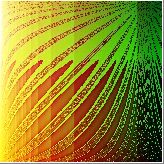
(ColorXY (sin (sin (+ (- (sin 0.151529) (tan -1.11426)) t))) (^ (% (cos u) (sin (/ (tan (^ u u)) (cos (log (sin (/ t t)) (log u (hsin t))))))) (+ (% (^ -2 (+ (sin t) (- u u))) t) t)) (- (sin (% (cos u) (sin (/ -0.6607 (cos (log (sin (/ t t)) (log u (hsin t)))))))) (* (/ (cos (/ t (+ u t))) (/ (- (- -1 u) -1) (log (* (cos t) (hsin (* (cos u) u))) t))) u)))
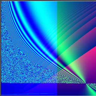
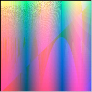
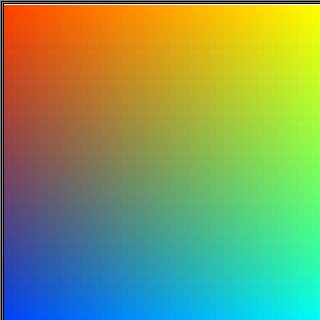
The other images are patterns that we think look nice that were created somewhere between generation 1 and 15.

(ColorXY (sin 0.267358) (^ (- (% (+ u (% (/ u 1.53775) -1.34795)) (sin (+ u (/ (% (+ u (sin (+ (- (sin u) (tan (% (^ (^ (/ -1.46619 -1) (tan 2.718)) -0.245224) (+ u (hcos (+ (cos (+ u (- (log 2.12837 u) t))) (* u (hsin (cos (cos (% 0.356211 (- -2.44942 (cos (/ u 2)))))))))))))) t))) (* (hcos t) (- (* u (sin t)) t))) t)))) u) u) (- 1 (sin 0.151529)))
(ColorXY (tan (% u (* t (- (* u (sin t)) t)))) (- (sin 1.43956) (cos (^ (hsin t) (tan (- (sin u) (tan (% (^ (^ (/ -1.46619 -1) (tan 2.718)) -0.245224) (+ u (hcos (+ (cos (+ u (- (log 2.12837 u) t))) (* u (hsin (cos (cos (% 0.356211 (- -2.44942 (cos (/ u 2)))))))))))))))))) (cos (sin (% 1.65267 (+ (hcos 0.373231) t)))))
(ColorXY (sin (- (/ (- t (hsin (cos t))) 0.219683) (cos (+ 2 t)))) (^ (- (% (+ u (% (/ u 1.53775) -1.34795)) (sin (+ u (/ (% (- (/ (- t (hsin (cos t))) 0.219683) (cos (+ 2 t))) (* (hcos t) (- (* u (sin t)) t))) t)))) -2.40397) u) (- -0.0434298 (+ (tan (* (cos u) t)) (tan (cos (- (% (+ u (% (/ u 1.53775) -1.34795)) (sin (+ u (/ 2.718 t)))) (sin (/ (tan (% u t)) u))))))))
(ColorXY (sin (sin (% (cos t) (sin (/ t 1.67288))))) (^ (% (cos u) u) (+ (% (^ -2 (+ (sin t) t)) t) t)) (- (/ (tan (^ u u)) (cos (log (sin (/ t t)) (log u (hsin t))))) (/ (sin (+ (- t (cos -1)) (tan (/ -3.07727 t)))) (^ (/ u (tan (+ u t))) (sin (* (sin u) -2.718))))))
(ColorXY u (- (tan -0.332632) t) (tan (+ u (sin -1.61549))))
Curve Fit
We also considered the problem of fitting a curve to a set of points. Our results were not as good for this problem. If the set of points fits a fairly simple curve, then the system would usually converge on this curve. However, if the points fit a complex curve that the system was not likely to guess, it did not do very well to find that curve or other curves with similar trends.
It did improve the fitness of the best program on each successive generation for a while. However, after many generations, it would usually get stuck converging on some curve with decent fitness that goes through about half of the points and goes nowhere near the others. It is difficult to break free from this convergence since all of the top programs look like it. It becomes necessary to increase the role of poorly fit programs in the hopes that some random mutation will help a lot
but this is not likely and does not work well. We believe we could obtain better results by choosing better ways of measuring fitness. We used only
distance of the curve from the points as a measure of fitness. Consideration of slope would have made the system aware of why some programs were better than the ones it calculated to be most fit.
Here is an example that worked fairly well. We chose 5 points along the curve y=x2-x+1 and used a population size of 100 programs. The programs displayed are the best fit programs for their respective generations. The fitness function we used was Sum(abs((fit_value - actual_value)) ^ 3 / actual_value). We cubed the distance between the fit point and the actual point to ensure that the fitted curve closely follows all the actual points, instead of hitting some exactly, but badly missing the others. Note that the solution evolved by us is not close to the actual curve from which we chose the points. This is not surprising because the curve it did find comes very close to the correct curve and thus has a high fitness. It is unrealistic to expect the system to find the exact same curve since its initial programs are random and some other curve may exist with very similar properties. In fact, other curves can exist that go through the same points, but have much different curvature. Since we are searching for any curve that goes through all points, these solutions are satisfactory.
Generation 1

(DefVarRange v0 1 1000 5)
(DrawXY ( v0) t (+ 6.15925 (cos (- 0.889367 (% (- t (- (hsin -0.90455) -1.51327)) t)))))
Generation 10

(DefVarRange v0 1 1000 5)
(DrawXY ( v0) t (* t (/ t 1.06113)))
Generation 37

(DefVarRange v0 1 1000 5)
(DrawXY ( v0) t (* t (/ (/ t 1.06113) 1.06113)))
Generation 64

(DefVarRange v0 1 1000 5)
(DrawXY ( v0) t (* (* (cos (sin -0.632015)) t) t))
Face Generation
The problems we encountered with the curve fit problem indicated that the more complex problem of face generation was not feasible without significantly more work. Due to time constraints, we did not consider this problem in detail.
To sum up, our system successfully evolved through the use of mutations and crossovers. Generally, the fitness of the best programs increased on each sucessive generation as expected. However, we encountered problems coming up with good selection criteria, a very important part of the system's success. Often the system would converge to a solution that was not close to optimal because that solution's fitness was significantly better than any other randomly generated solutions. Sometimes this was because the other random solutions were really bad, but sometimes it was because our method of measuring fitness did not consider all aspects of what makes a progam fit. Another issue we found was that the system's performance was closely tied to the parameters we used for evolution, program generation, mutation, and crossover. This presents an undesirable situation where the settings for every problem must be carefully calibrated in order for the system to have any success solving that problem. Experimentation with measuring fitness and with the system parameters are essential for creating a successful evolutionary programming system.
1. Artificial Evolution for Computer Graphics, Karl Sims, Computer Graphics, Volume 25, Number 4.
2.Genetic Algorithms as Tools for Creating "Best-Fit" Parametric Surfaces, Aravind Narasimhan and Hersh Reddy, Cornell University, 1995.
3. The Origin of Species, Charles Darwin, 1859.