Central pattern generator/double
pendulum model
Bionb
2220, CI Section, 4/27/09
By: Devin Cowan
Simple spring-mass systems are all around us. Harmonic
oscillators have been used to explain everything from the vibration of valence
electrons to the “travel” of a bike’s suspension system. This model explores
the interaction simple neural networks with dynamical systems whose behavior is
based on simple harmonic oscillators. In particular, I used computer simulation
to observe the interaction of central pattern generators and the motion of a
double pendulum.
Background:
Central pattern generators (CPG’s)
are clusters of interneurons found in both vertebrates
and invertebrates (Tytell). These relatively simple
neuron networks are capable of synchronizing and producing rhythmic patterns
thought to drive repetitive motor movements (Hooper 1). Several studies have
demonstrated that oscillatory motor output CPG’s can
entrain to an energy efficient frequency of firing when receiving sensory
feedback (Iwasaki and Zheng 1). Certainly, it seems
that CPG’s will inherently “seek” an energy minimum
provided suitable parameters (gain, saturation). However, this has only been
demonstrated using single-degree-of-freedom systems; in other words, most
studies have modeled the physics of motor output as a simple point-mass
pendulum or a spring-mass oscillator (Verdaasdonk,
Hatsopoulos).
Methods:
This study was an attempt to create a more physically
realistic model of a CPG/limb system. The primary difference between this and previous
work is the use of a double pendulum (Figure 1) rather than the “limbs”
mentioned above.
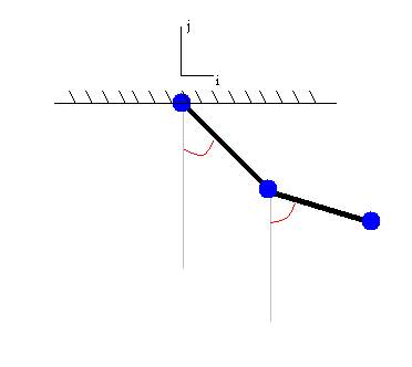
Figure 1: Double pendulum,
2-DOF
Using this novel model, I wanted to observe the limb
behavior for different parameter settings and initial conditions. I thought
that some interesting patterns, like those in other 2-DOF systems, might arise.
Figure 2 shows one such pattern—the displacements of two masses as they are
forced near one of the system’s eigenvalues (a normal
mode frequency).
Figure 2: Oscillations of a
2DOF system that is forced near its natural frequency
In addition to introducing a second degree of freedom, the
double pendulum system necessitated the use of two central pattern
generators—one driving each set of flexor and extensor muscles (each joint,
“elbow” and “shoulder” had one such set of muscles). Figure 3 is a connection
diagram for the model, modified from Iwasaki and Zheng.
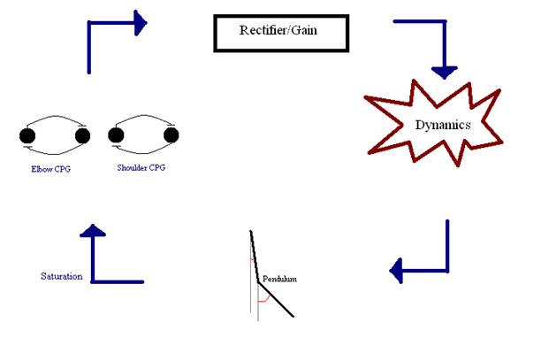
Figure 3: Flow diagram for model system—two CPG’s and a double pendulum
The CPG’s were both modeled using Izhikevich’s
numerical integrator. Each consisted of two reciprocally inhibiting neurons,
whose output was rectified (to account muscle contraction, as opposed to active
extension) and amplified before driving the motion of the pendulum.
A great portion of my efforts were spent on determining the equations of motion for the double pendulum, and implementing them in such a way that they could be numerically integrated within Izhikevich’s construct (which uses a Euler’s Method type integrator). The equations were determined using angular momentum balance about hinge points. Inertial terms were not neglected. A damping moment, proportional to the angular velocity of the limb segment, was accounted for at the “elbow” and “shoulder” joints. Neural output from the CPG’s was implemented as a direct moment about each of the joints. For further details, follow Ruina and Pratap’s similar example of a robotic arm (930).
Because the dynamics of the physical model are complex, this model was tested in standalone before addition of the CPG’s. Figure 4 shows one such test, in which the double pendulum was released with no initial velocity. As expected of a damped oscillator (note that both joints were damped), the system’s motion eventually ceases.
Figure 4: Motion of a double pendulum agitated at t=0, without neural interaction
Similarly, the behavior of the CPG neurons before addition of sensory feedback was recorded (Figure 5).
Figure 5: Behavior of CPG’s without feedback from the pendulum
Results:
With a baseline set of data in hand, I enabled driving and feedback in the CPGs. Using parameters from Iwasaki and Zheng, the CPG/pendulum system was scaled up to its full connectivity. Below are several of the outputs:
Figure 6: Rod positions during CPG activity (dt=.01, tend=200, gain=1)
Figure 7: CPG activity with feedback
Figure 8: positions during CPG activity (dt=.01, tend=500, gain=1)
Figure 9: CPG activity with feedback (over a long period)
Figure 6-8 show incredibly huge (not to mention physically impossible) position values for the two rods of the double pendulum. I quickly found that this could be remedied by decreasing the gain (Iwasaki and Zheng witnessed entrainment for gain~1). However, the decreased gain resulted in still other problems—radical shift patterns like that of Figure10 were observed at low gain values.
Figure 10: Radical shifting pattern of mothion
The abrupt spiking in Figure 10 diminished upon integration with a smaller step size.
Figure 11: Small step size integration
Discussion:
Despite that the results in Figure 11 closely resemble the motions of a near-harmonic 2-DOF system (Figure 2), replication of other such patterns (and verification that they aren’t simply artifacts of the parameters and integration times) was hindered by several constraints:
- The dynamics of the double-pendulum require inversions of large state matrices. This inversion and reallocation is carried out at every time step, making numerical integration by the Euler Method bulky and computationally intensive (most of the computers I ran code on were unable to integrate over more than 200ms without freezing).
- Since the model can only be integrated over small time scales, recognition of long-run patterns (one of the goals of the study) was close to impossible.
- Increasing the time-step in order to view long-range predictions causes a high degree of error in the integration. This error is propagated by the method of integration, resulting in wildly inaccurate limb behavior. Such inconsistencies again render long-term modeling unproductive
Despite that my goal of searching for oscillatory limb patterns was obviated by my choice of computer model (and its computational demand), I feel that this project has other contributions. I hope that my painstaking double-pendulum implementation might prove useful in other models, if in no other way than by raising the standard of modeling from “spherical chickens” to spherical chickens that have joints!
References:
Hatsopoulos, Nicholas G. Coupling
the Neural and Physical Dynamics, Neural Computation 1996, 8, 567-581.
Hooper, Scott L.
Central Pattern Generators. Embryonic ELS 1999, 1-12.
Iwasaki and Zheng. Sensory
feedback mechanism underlying entrainment of central pattern generator to
mechanical resonance, Bio. Cybernetics 2006, 94:245-261.
Izhikevich, Eugene. Simple
Model of Spiking Neurons, IEEE Transactions on Neural Networks (2003)
14:1569- 1572 (electronic resource: <http://vesicle.nsi.edu/users/izhikevich/publications/spikes.htm>).
Ruina, Andy and Pratap,
Rudra. Introduction to Statics and
Dynamics. Pre-release version for Oxford University Press: 2008.
Tytell, Eric. The Benefits of Positive Feedback, Journal of Experimental Biology 2007, iv.
Verdaasdonk, B.W. Energy efficient and robust rhythmic limb movement by central pattern generators, Neural Networks 2006, 19: 388-400.
Code:
%%%%%%%%%%%%%%%%%%%%%%%%%%%%%%%%%%%%%%%%%%%%%%%%%%%%%%%%%%%%%%%%%%%%%%%%%%%
% Neural
Network Simulator
% Using models from Izhikevich
%
http://nsi.edu/users/izhikevich/publications/spikes.htm
% Bruce
Land -- BioNB 222, March 2008
%
Additional edits by Devin Cowan April 2009
%%%%%%%%%%%%%%%%%%%%%%%%%%%%%%%%%%%%%%%%%%%%%%%%%%%%%%%%%%%%%%%%%%%%%%%%%%%
function izRob()
clf
clear all
clc
% Number
of neurons
nNeuron = 4 ;
% Number
of Sensory cells
% In this version they must be equal
nSense = nNeuron;
%timing
dt = .01; %time step
tEnd = 200; %maximum simulation time
%build the time vector
time = 0:dt:tEnd ;
%CPG and
dynamics parameters
q=.4; lam=2; %Used for
saturation feedback function
sDamp=10; %Damping
coefficient in the shoulder
eDamp=10; %Damping
in the elbow
l1=4; l2=3; %Half
length of the upper and lower leg
l3=2*l1; %The com is centered on the first section
m1=30; m2=15; %Mass of
limb segments
g=9.8; %Gravitational
constant
ihat=[1;0;0]; jhat=[0;1;0]; khat=[0;0;1]; %Frame basis vectors
I1=1/12*m1*(l1*2)^2; %Moment of inertia
I2=1/12*m2*(l2*2)^2;
%cell
parameters from Izhikevich web page. See:
%
http://nsi.edu/users/izhikevich/publications/spikes.htm
% a
b c d
current
pars=[0.02 0.2
-65 6 14 ;...
% tonic spiking
0.02
0.25 -65 6
0.5 ;...
% phasic spiking
0.02
0.2 -50 2
15 ;...
% tonic bursting
0.02
0.25 -55 0.05
0.6 ;...
% phasic bursting
0.02
0.2 -55 4
10 ;...
% mixed mode
0.01
0.2 -65 8
30 ;...
% spike frequency adaptation
0.02
-0.1 -55 6
0 ;... % Class 1
0.2 0.26
-65 0 0 ;... % Class 2
0.02
0.2 -65 6
7 ;... % spike latency
0.05
0.26 -60 0
0 ;...
% subthreshold oscillations
0.1
0.26 -60 -1
0 ;... % resonator
0.02
-0.1 -55 6
0 ;... % integrator
0.03
0.25 -60 4
0;... % rebound spike
0.03
0.25 -52 0
0;... % rebound burst
0.03
0.25 -60 4
0 ;... % threshold variability
1
1.5 -60 0
-65 ;... % bistability
1
0.2 -60 -21
0 ;... % DAP
0.02
1 -55 4
0 ;... % accomodation
-0.02
-1 -60 8
80 ;...
% inhibition-induced spiking
-0.026
-1 -45 0
80]; %
inhibition-induced bursting
%extract the cell type for each neuron
nType = [3 3 3 3] ;
a=pars(nType,1)';
b=pars(nType,2)';
c=pars(nType,3)';
d=pars(nType,4)';
Is = pars(nType,5)'; %steady current
%synaptic
connections
%The
weight matrix -- (+)excitatory: (-)inhibitory
SynStrength =10*[0 -.5 0 0;
-1 0 0
0;
0 0 0 -.5;
0 0
-1 0] ;
%each
neuron also potentially has several sensory inputs
SenseStrength =[1 0 0 0;
0 1 0 0;
0 0 1
0;
0 0 0 1];
%Sense
inputs are time vectors on the inputs--DIRECT INPUTS from experiment
SenseInput(:,1) = 10*
(time>5 & time<10);
SenseInput(:,2) = 0 * (time>5
& time<10);
SenseInput(:,3) = 10 *
(time>5 & time<10);
SenseInput(:,4) = 0 *
(time>5 & time<10);
%synaptic
current rises instantly, then decays exponentially
%set the
decay rate of synaptic current to about 3 mSec
SynRate = .3*ones(1,nNeuron);
SynDecay = 1 - SynRate*dt;
%init
state variables
v = c; % reset
voltage;
s = zeros(1,nNeuron); % spike occurance
u = zeros(1,nNeuron); % revocery
variable
%initial
input currents
Istate = 0; %state
variable used for synaptic currents decay
I = Is ;
%step the
time
tindex = 1; %pointer for output arrays
%init
plotting variables
Vout = zeros(length(time),nNeuron);
Aout = zeros(length(time),nNeuron);
THout=zeros(length(time),6); %1&2
are theta vals, 3&4 are thetadot
vals
th=zeros(1,6);%Initialize
theta values...0=leg starts downward
M=[0 0;0 0]; %Dynamics matrix used for calc of ang. accelerations
RHS=[0;0];
%%%%%%%%%%%%%%%%%%%%%%%%%%%%%%%%%%%%%%%%%%%%%%%%%%%%%%%%%%%%%%%%%%%%%%%%%%%
%MAIN
%%%%%%%%%%%%%%%%%%%%%%%%%%%%%%%%%%%%%%%%%%%%%%%%%%%%%%%%%%%%%%%%%%%%%%%%%%%
for t=time
%add values to plotting variables
Vout(tindex,:)=v;
Iout(tindex,:)=I;
THout(tindex,:)=th;
%DO DYNAMICS--assign vals to th
ms=detMoment(v(1:2)); %Find the moments based on the v's
me=detMoment(v(3:4));
tTemp=th(1:2); tdTemp=th(3:4); tddTemp=th(5:6); %Unpack vars
%Differential equations
th(1:2)=tTemp+dt*tdTemp;
th(3:4)=tdTemp+dt*tddTemp;
%Angular momentum ballance to calc. angular accelerations
lam1=sin(tTemp(1))*ihat-cos(tTemp(1))*jhat; %Unit vercots along the two sections
lam2=sin(tTemp(2))*ihat-cos(tTemp(2))*jhat;
%Define various physical
parameters
rg1o=l1*lam1; rg2e=l2*lam2; reo=l3*lam1;
rg2o=reo+rg2e;
sumMe=cross(rg2e,-m2*g*jhat)+me*khat-eDamp*tdTemp(2)*khat; %RHS of AMB
sumMs=cross(rg1o,-m1*g*jhat)+cross(rg2o,-m2*g*jhat)...
+ms*khat-sDamp*tdTemp(1)*khat; %Damping prop. to
angular velocity
T1=cross(khat,reo); T2=cross(khat,rg2e); T3=tdTemp(1)^2*reo+tdTemp(2)^2*rg2e;
M(1,1)=dot(m2*cross(rg2e,T1),khat);
M(1,2)=dot(m2*cross(rg2e,T2)+I2*khat,khat);
addE=m2*cross(rg2e,T3);
RHS(1,1)=dot(sumMe+addE,khat);
T4=-tdTemp(1)^2*rg1o; T5=cross(khat,rg1o);
M(2,1)=dot(m1*cross(rg1o,T5)+I1*khat+m2*cross(rg2o,T1),khat);
M(2,2)=dot(m2*cross(rg2o,T2)+I2*khat,khat);
addS=-(m1*cross(rg1o,T4)-m2*cross(rg2o,T3));
RHS(2,1)=dot(sumMs+addS,khat);
th(5:6)=inv(M)*RHS; %Invert M to calculate the angular
accelerations
%input current to cells
%decaying synaptic currents
Istate = s*SynStrength + Istate .* SynDecay ;
%Sensory inputs (direct and from
muscle mechanoreceptors)=saturation(th)
saturation=q*tanh(lam*th(1:2)); %Two sat vals, one for each limb seg.
sat=[saturation(1)
-saturation(1) saturation(2) -saturation(2)]; %All neurons are driven
directly by mechano.
SenseInput(tindex,:)=SenseInput(tindex,:)+ sat;
I = Istate + Is + SenseInput(tindex,:)*SenseStrength;
%update state variables
v = v + dt
*(0.04*v.^2+5*v+140-u+I); %Neural ODE's
u = u + dt * a .* (b.*v-u);
s = zeros(1,nNeuron)
;
fired=find(v>=30);
%
indices of cells that spiked
if ~isempty(fired)
v(fired) =
c(fired) ;
u(fired) =
u(fired)+d(fired) ;
s(fired) = 1 ;
%used
in the next time step for synaptic input
end;
%update time index
tindex
= tindex+1;
end %main time
step for-loop
%Plot the
CPG activity
figure(1)
clf
np=nNeuron ;
for i=1:nNeuron %Plot the currents and voltages of
the neurons
subplot(np,1,i)
plot(time,Vout(:,i))
hold on
plot(time,Iout(:,i),'r')
plot(time, SenseInput(:,i)*SenseStrength(i,:), 'g')
ylabel(num2str(i))
set(gca,'ylim', [-100 50])
end %Neuron
plotter
%Plot the
position over time
figure(2)
plot(time,THout(:,1),'g',time,THout(:,2),'r')
xlabel('time'); ylabel('theta (radians)')
%Call the
animation function
leg(THout(:,1),THout(:,2),time,2*l1,2*l2)
%Animate
a leg
end %of iz
function
leg(th1,th2,time,l1,l2)
%Takes
post-integration theta values and animates them
for i=1:length(time);
e=l1*[sin(th1(i)); -cos(th1(i))];
h=e+l2*[sin(th2(i)); -cos(th2(i))];
upper=[[0;0] e];
lower=[e h];
x1=upper(1,:);
y1=upper(2,:);
x2=lower(1,:);
y2=lower(2,:);
figure(3)
pause(time(2)-time(1))
plot(x1,y1,x2,y2)
axis('equal');
axis([-10 10 -20 5]);
end
end
function M=detMoment(v)
%Determines the moment to apply, given the two voltages of
the CPG
gain=1;
M=gain*(max(v(1),0)-max(v(2),0));%neuron 1 applies as positive
moment
end %Of detMoment