An Event Based Neuron Network Model

By Pavel Sountsov

Introduction

There are two primary methods of simulating complex neural networks. One is to describe each neuron as a set of time dependent differential equations, and then simulate the system by advancing the time by either a fixed or a variable timestep. The other method involves solving those differential equations and then using those solutions to advance the system to the next state discontinuity, such as the spiking of a neuron.

The timestep method has the advantage of being relatively easy to simulate and formulate. In terms of formulation the differential equations can be obtained from mathematical analysis of the phase diagrams of neurons that are being simulated, or voltage clamp recordings of individual ions in biological neurons. The simulation can proceed through the use of Euler or Runge-Kutta integration methods, preferably using the implicit versions of those algorithms for greater stability of the often stiff systems. A disadvantage of this method is that, if the timestep is large enough, the quantization of the simulation may adversely affect neural nets where spike timing is of importance. To prevent that small timesteps are often used, but this leads to computational inefficiency because many more calculations have to be done.

The event based method has the advantage of the complete lack of quantization of the simulation. Each event, each spike happens at the exact time it is supposed to happen given the system description. Also if the system is quiescent, that is, the ratio of times of inactivity to the times of activity is relatively high, the simulation speed can be greatly increased. This depends on the system however, and since this method requires more computation per system update this favourable ratio can often not be achieved. A great disadvantage of this method is that the closed form solution of the differential equations is often impossible. In fact, no biologically realistic neuron is simple enough to solve analytically. Simpler neurons, such as the integrate and fire neuron, however, can be solved and thus benefit from this method immensely. In the end, if these disadvantages are surmounted, this method is almost always preferred.

One disadvantage of the integrate and fire neurons is that they do not exhibit too many of the features of realistic neurons, such as bursting, variable threshold et al. Thus, a more complicated model is preferred.

Model Description

For this project I sought to create an event based simulation of a slightly more complicated neuronal model. Since it is far easier to tweak the model while running the simulation using the timestep method. The model has three state parameters: V, a, I. V roughly represents the membrane potential of the cell. a governs the second-dimensional features of the model such as bursting and spike rate adaptation. I represents the decaying synaptic current. In addition to the state variables, the system is described by 11 more constants, which are letters K, L, M, N, P, D, C, E, F, Ic and d. Aside from Ic, which represents the constant current input into the cell, the constants' meaning is somewhat abstract. The equations that describe the system are as follows:

V' = -KV + Ic + I - a
a' = -M if a > N (Ic + I)
a' = M if a < N (Ic + I)
I' = -d if I > 0
I' = d if I < 0

Also, there are two threshold based state switches. One for V:

if V > P then
V = D
a = a + F

And one for a:

if a > C
a = E

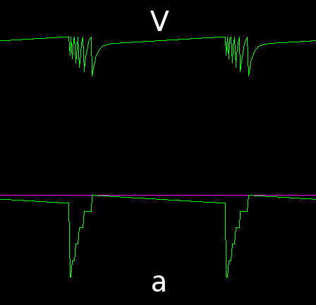
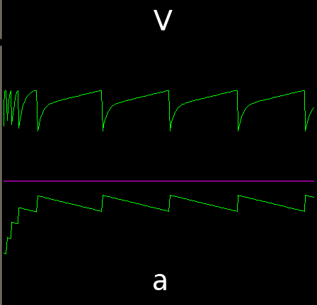
The model can replicate many styles of spiking, such as tonic and phasic spiking, tonic and phasic bursting and others. Seemingly this model does not produce nice spikes after it reaches threshold, but through testing of biologically realistic systems it was found that the exact behaviour of the system during the spike is of limited importance. Thus, if the one so prefers, one can add some vertical lines at the spike times. Here are some sample traces from the model.

To convert this model to an event based simulation method, one has to solve all of those differential equations. This process is a little complicated, but doable. For completeness's sake the full form solutions are as follows. Note that two new variables are introduced, curd and curM, which represent the current values of d and M, given the value of I and a respectively (see the state descriptions above). Also, there is are a set of free variables that depend on the initial conditions, these are O, a0, I0. t is the independent variable. e is the base of the natural logarithm.

V = (curd - a0 K + I0 K + Ic K - curM) / K^2 + (curM - curd) t / K + O e ^ (-K t)
a = a0 + curM t
I = I0 + curd t

The event based simulation method depends on solving those equations for specific times at which the equations above change their form. Besides the two threshold transitions that are present in the model, there are two more state changes. Also, the equations must be updated each time the I is increased due to the synaptic input from another cell. Namely, the times when curM and curd change sign. This leads us to a total of 5 times that are generated at every model update, one time for each future event change. Thus, the general modus operandi of the model would be to find all of those 5 times, then pick the one that happens the soonest, update the time by that amount, find the 5 times again and so on. The exact formulas won't be provided, and can be examined within the model implementation. .

Normally, an event queue would be used, but for this particular implementation a simpler method is used. Each cell is updated at a fixed time interval, while keeping track of the time elapsed since the last event. An model update is triggered once the time elapsed matches or exceeds the time obtained from the previous event update.

Sample Neural Network Implementation

To test this model a simple network simulating the cerebral cortex was created. It consists of 1000 of interconnected cells. One fifth of them are faster spiking, inhibitory cells. The rest are slower, excitatory cells. Each cells is connected to 5 other cells randomly choses from the neuron population. Also, the cells are set to get random current injections, simulating the input from the basal ganglia. The C++ source code implementation is given below.

Download Sample Implementation

This network exhibits some rhytmic activity as can be seen from the images.