Simulating ELa and ELp Responses

Bruce Land, Carl Hopkins, Lauireanne Dent

Introduction

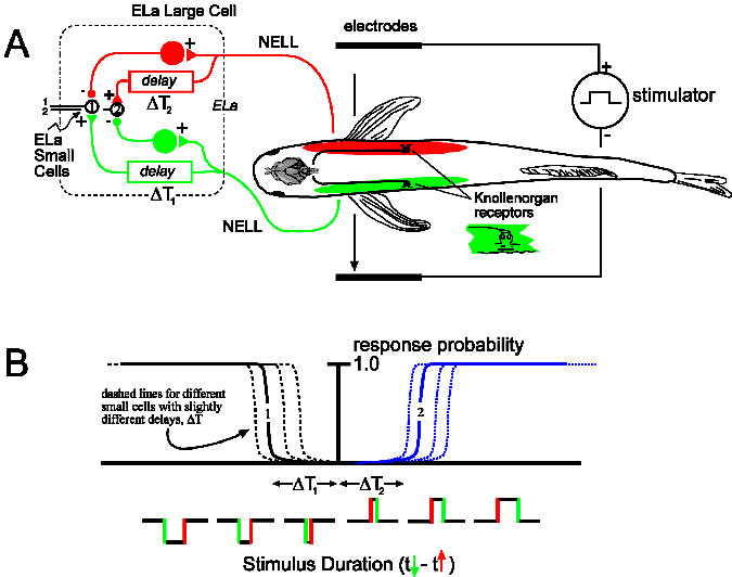
Mormyrid fishes recognize the sex and species of other fishes by their electric organ discharge waveforms (EODs). These signals are encoded with microsecond precision by peripheral Knollenorgan electroreceptors ( KOs) which project to a dedicated time-coding pathway in the brainstem. One model proposes that stimulus-evoked spikes, originating in two different regions of the skin, will arrive at small cells in the anterior exterolateral nucleus (ELa) via both an excitatory input which is delayed and an inhibitory input with a shorter delay. Only stimuli with durations exceeding the conduction time of the axonal delay line (i.e., the excitation due to the pulse onset traverses the axonal delay before the inhibition due to the pulse offset arrives) will excite the ELa small cell (for example, cell 2 in figure ‘A’ with long duration stimuli). If all KOs are stimulated simultaneously, inhibitory inputs should arrive first, preventing the excitation of small cells.

This model has been tested by stimulating Brienomyrus brachyistius KOs with head-tail or transverse electric field geometries designed to stimulate receptors sequentially, and uniform geometry designed to stimulate them synchronously while recording in vivo evoked potentials from the posterior exterolateral nucleus (ELp), the sole recipient of ELa small cell output. Given that electric field strength was sufficient to drive “all” KOs, we predicted no evoked potentials in ELp under uniform geometry compared to a large evoked potential under head-tail and transverse geometry.

To interpret this experiment, a simulation of certain elements of the neural network was performed. The next sections outline the simulation and some results.

Xu-Friedman MA, Hopkins CD (1999)

Simulation Assumptions

• A simplified geometric model of a fish body was constructed with four isopotential quadrants, each with a specified number of electrorecptors. Electric fields are assumed to be applied left/right or front/back with either polarity, or uniformly across the entire body.
• About 100 receptor cells are used, modeling the actual number on a fish. Each electroreceptor consists of a linear convolution filter and a rectifier, followed by a spike generation scheme:
  • The filter and rectifier transduce a voltage into a current that will directly control the probability of firing a neuron.
  • Each electroreceptor has independently settable parameters for filtering, time constant, threshold and threshold noise. The filter center frequencies are log-normal distributed. For the front half of the fish the mean frequency was 1500 Hz, with a range of 200 to 4000 Hz. The distribution used was exp(log(1500)+randn*0.55). For the back half of the fish the mean frequency was 2000 Hz, with a range of 1500 to 2500 Hz. The distribution was exp(log(2000)+randn*0.18). The function randn returns a normally distributed number with mean zero and standard deviation one.
  • The distribution of center frequencies as used to construct butterworth bandpass filters with a lower cutoff of (cf-cf*0.8) and a higher cutoff of (cf+300) where cf are the center frequencies from the step above. These particular values were chosen to approximate the shapes of the response curves from actual fish.
  • The output of each receptor was a spike train. The probability of firing is a free parameter and was set to 0.05 per time step per unit input current. There was a refractory period during which a spike could not occur. This was set to 1.2 mSec based on Bell and Grant (1989).
• The output of the receptor cells go through a simplified pathway, modeled by delays, to small cells in the ELa. About 1000 small cells were modeled. Each small cell was modeled as an integrate-and-fire with delayed inputs from the receptors:
  • Each small cell had two inputs, picked at random from all receptors. One excitatory, one inhibitory.
  • Delay assumptions:
    • First Pass:
      • The inhibitory input had a delay chosen from a normal distribution with mean of 56 microSec, standard deviation of 11 microSec, and with a minimum of 10 microseconds. (Friedman and Hopkins 1998, measured by Laurieanne)
      • The excitatory input had a delay chosen from a normal distribution with mean of 386 microSec, standard deviation of 52 microSec, and with a minimum of 10 microseconds. (Friedman and Hopkins 1998, measured by Laurieanne)
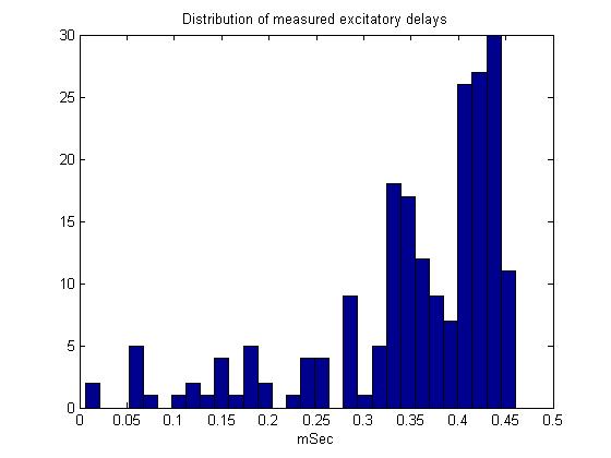
    • Second pass. There is a long tail on the excitatory delay distribution toward low delay. this tail was explicitly inculded in the model.
      • The inhibitory input had a delay chosen from a normal distribution with mean of 56 microSec, standard deviation of 11 microSec, and with a minimum of 10 microseconds. (Friedman and Hopkins 1998, measured by Laurieanne)
      • The excitatory input had a delay chosen from the actual measured distribution. (Friedman and Hopkins 1998, measured by Laurieanne)
  • The strength of the inhibitory input is much greater the the strength of the excitatory input. The strength of the excitatory input is just sufficient to reach threshold with a single AP input. The duration of the simulated synaptic current approximates the time course in the real cells. The current rises quickly then falls exponentially.
  • There is a refractory period after a spike. The membrane potential is reset to rest after a spike.
• The spike trains are convolved with a narrow Gaussian, summed across cells for each time, and plotted to approximate the observed field potential from the ELa and ELp.

Program

A Matlab program was written to implement the simulation. All of the receptor cells are simulated, the spike trains stored in a compressed format, then all of the small cells are simulated. There are options to build a new fish or to just apply a new stimulus to a fish which was already built. Output plots appear in 3 figures:

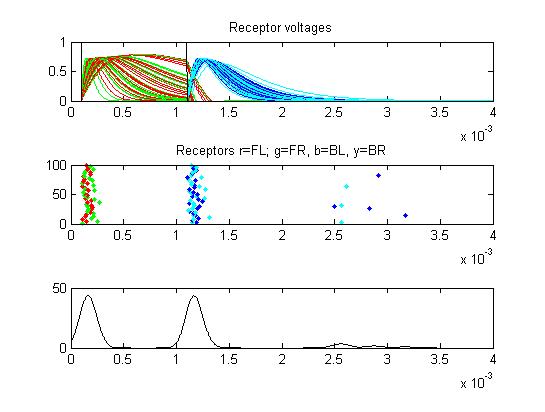
• Receptors: receptor currents, spikes as a raster plot and summated spikes.
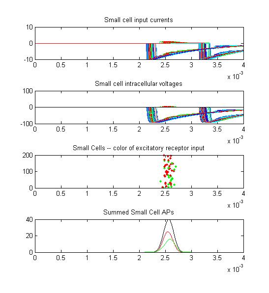
• Small cells: input currents, membrane voltage, spikes as a raster plot and summated spikes.
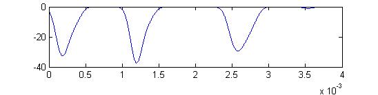
• Sum of receptor and small cell spikes, which simulates the traces that Laurieanne records.

The following examples show the model performance under several conditions. All of these examples were run with just 200 small cells, not the usual 1000. All simulations were on the same 'fish'.

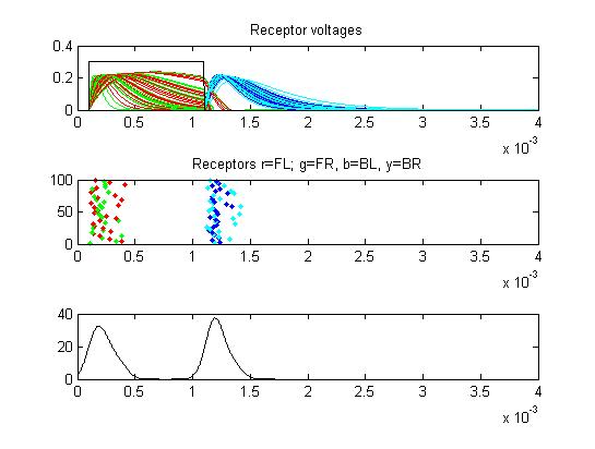
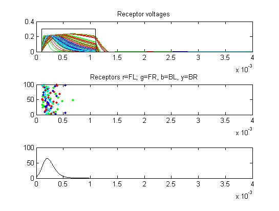
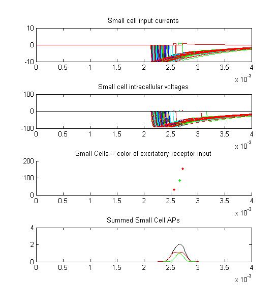
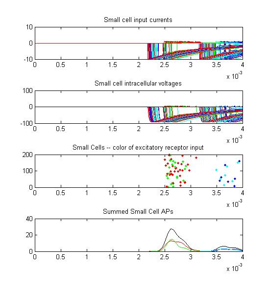
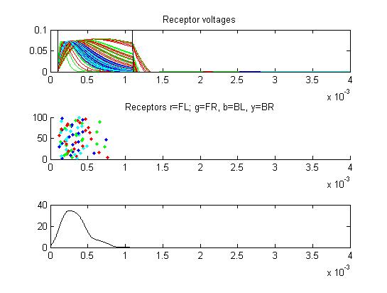
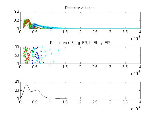
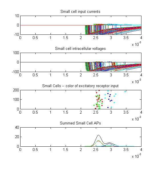
1. The first example is a relatively long stimulus of 1 mSec, medium amplitude (0.3), and head/tail field orientation. Note the different duration receptor voltages depending on the center frequency of the convolution filters. Receptor spikes are bunched around the onset (head receptors) and fall (tail receptors) of the stimulus.
   
   Small cell input currents below show the size ratio between the large inhibitory and small excitatiory inputs and also show that the excitation is delayed relative to the inhibition. Inhibition is long lasting, so there is only one burst of output spikes.
   
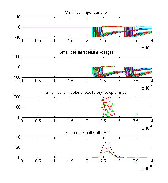
   Summed APs. This figure is an approximation of recordable data. Note that the relative weighting of the receptor and small cells amplitudes may be wrong.
   
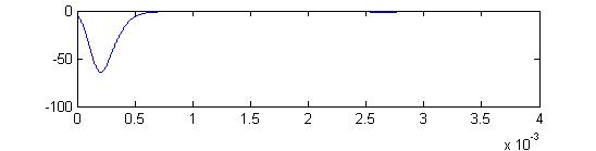
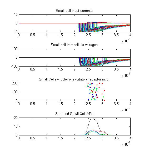
2. The second example is a relatively long stimulus of 1 mSec, medium amplitude (0.3), and full-body field orientation. this is the same stimulus as example 1, but is applied to the entire body. Note that virtually all the receptors fire on the rising edge of the outside-positive pulse.
   
   Only two or three small cells escape from the massive inhibition caused by all the receptors firing at once.
   
   There is only the smallest AP distribution from the small cells.
   
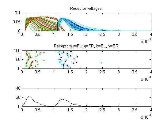
3. The third example is a relatively long stimulus of 1 mSec, low amplitude (0.1), and head-tail orientation. The lower stimulus, combined with the variablity of the convolution filters causes the receptor firing to become multimodal.
   
   
   
4. The fourth example is a relatively long stimulus of 1 mSec, low amplitude (0.1), and full-body orientation. Again, the lower stimulus, combined with the variablity of the convolution filters causes the receptor firing to become multimodal.
   
   Because less than 1/2 of the receptors produced an AP, some of the small cells avoid inhibition and fire.
   
   
5. The fifth example is a relatively long stimulus of 1 mSec, high amplitude (1.0), and head-tail orientation.
   
   Note the full supression of the second AP peak below.
   
   
6. The sixth example is a relatively short stimulus of 0.2 mSec, medium amplitude (0.3), and head-tail orientation. The receptor output is multomodal for a different reason: The rising edge and falling edges overlap.
   
   
   

Possible comparisions between simulation and data

1. Qualitatively, both the simulation and the data show a block in ELa output for high amplitude, full-body stimulation. The model predicts less block for head-tail stimulation than the real data at high stimulus amplitude.
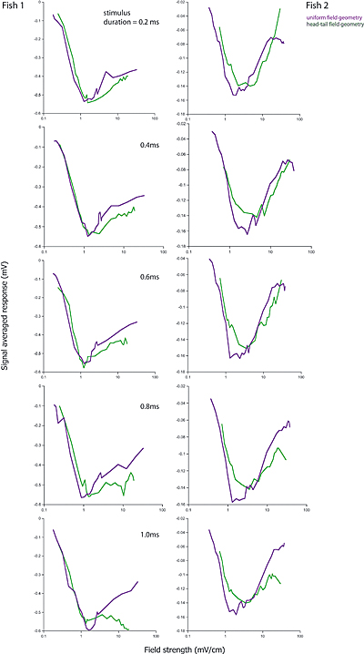
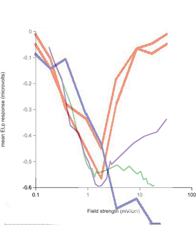
2. Laurieanne's data shows that on a plot of evoked potential amplitude versus stimulus amplitude, the biggest response occures at a specific stimulus amplitude (which depends on the fish), independent of the stimulus duration. In the following, fish1 is left, fish2 is right.
   Duration is 0.2 mSec at top and 1.0 mSec at bottom. Purple is full-body, green is head-tail.
   
   A simple interpretation of this could be: At low stimulus, response amplitude should be proportional to stimulus amplitude because to takes only one receptor to fire a small cell, but concidence with an inhibitory cell to stop firing. For full-body stimulation the response amplitude should go as n*(100-n) where n is the number of responding receptors. If n is proportional to stimulus amplitude (and not duration), there will always be a peak at about 50% activation. The first-pass model does not predict this independence of stimulus duration. This is because the probability of receptor firing is proportional to (stim strength)x(stim duration), not just to the strength. Adding an extra delay to the inhibitory small cell inputs seems to fix this problem (item 2 below). The extra inhibitory delay allows a few excitatory inputs to 'leak through' the inhibition at higher stimulation strength. The second-pass model (item 3 below) partly fixes the problem in a more natural way, by taking into account the long tail on the excitatory delay distribution shown here.
   
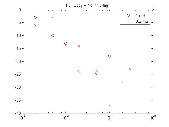
   1. For the first pass case (described in the assumptions above), the biggest response moves to higher amplitude at shorter stimulation duration.
      
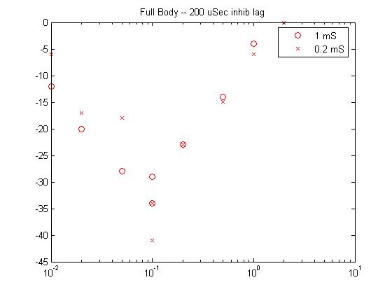
   2. If 200 microseconds extra delay is added to the inhibitory inputs (program), then the stim/response curves look like Laurieanne's. The different duration curves overlap. And the slopes are similar to real data.
      
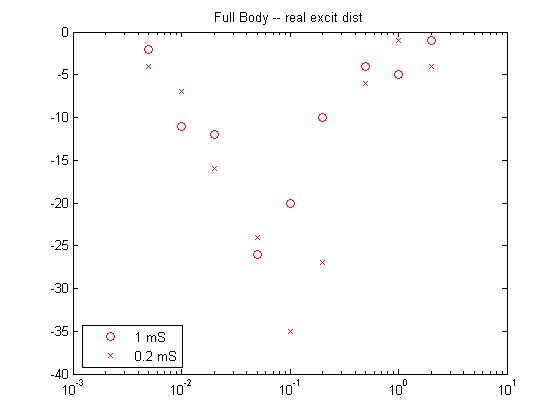
   3. For the second pass case (described in the assumptions above), the real distribution of excitatory delays was used (program and datafile of all delays) . The resulting response curves look promising, but the shift in the peak amplitude suggests that there probably needed to be more modeled delay in the inhibitory inputs. the slopes are good, particularly the curvature of the response curve at high amplitude, which resembles real data.
      
   4. A modification of the second pass added 30 uSec of delay to the inhibitory side. The resulting response curves match the real data fairly well, however The head-tail stimulation flatttens out at a lower level.
      
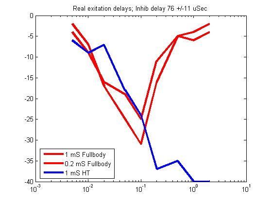
      Overlay onto real data. Purple is fullbody, green is head-tail. Note that the horizontal scale was stretched to match one decade. Vertical scale was stretched to approximate peak-to-low value ratio. Model was translated to match peak positions.
      
3. Ratio of ELa to ELp peak amplitudes may constrain the simulation.
4. Multimodal peaks in receptor response may constrain amplitude-center frequency relationship.

This section added after the Journal Club. Added on: 17 May 2006

Fitting real data

We wrote a modifed program which automatically generated strength-response curves. Laurieanne compared these to real data and found a good fit with an inhibitory delay distribution of mean=250 microsec and std.dev=125. The following plots show a case computed with a Gaussian distrbution of inhibitory delays with mean=206+/-61 microseconds. Pulse length was set to 200 microseconds. Four separate fish were generated to check for the effect of random variation due to filter responses and small cell wiring. Horizontal scale is stinulus strength, vertical is peak of simulated evoked potential. (this program generates detailed currents and voltages)

Can the model resolve distance and direction?

A real fish needs to be able to untangle the effects of amplitude and EOD phase to determine the direction of another fish, independently of the distance to the fish. Distance scales the EOD waveform, therefore changing its effect on nonlinear receptors in a complex way. Ideally, the outputs from the small cells should be able to separate the distance from the direction. There are several considerations:

• A simple assumption is the the small cell inputs extract all of the timing information for the EOD, and that duration/refractory period limits any small cell to only one spike.
• Since any one small cell can emit either one or zero spikes, then the output can be represented as a binary digit, and the output of all the small cells can be written as a binary string in some arbitrary order.
• No matter what decoding scheme is used by the fish on small cell outputs, there must be a difference in the pattern of firing (the binary string) which is detectable.
• The simplest measure of the difference between two binary strings is the Hamming Distance (HD). The HD is defined as the number of nonmatching digits of the binary string. The HD has some nice properties. For a fixed number of small cells, it is a metric. This means that a cell always has zero HD from itself, it is non-negative, it is symmetric, and it obeys the triangle inequality.
• If we apply different amplitude (distance) and phase (direction) model stimuli, then compute the HD between every pair of responses we can ask questions like "Are all of the different amplitude responses from one direction nearer to each other than to other directions". You would hope that directions would cluster in terms of HD.

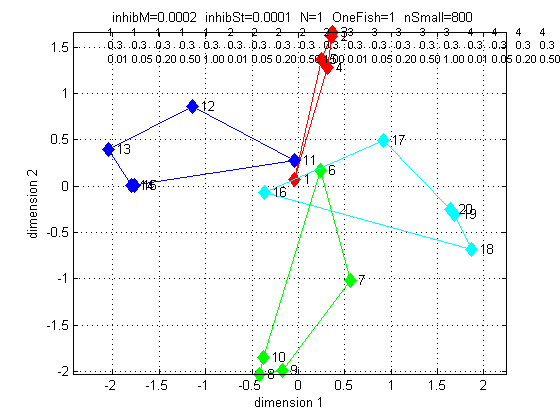
The program presents 20 stimuli to a model fish with 100 receptors and 800 small cells. The 20 stimuli are broken down into 4 directions, each presented at 5 amplitudes. Clustering of HD was initially done by looking at a table, but patterns are hard to see, so a technique called Multidimensional Scaling (MDS) was used to lower the dimensionality. You would expect range/phase data to be two dimensional, since there are just two parameters. So the question comes down to whether the 20-dimensional HD data set fits into two dimentions in an understandable way. The following plots shows that it does. The pulse duration matched the average EOD duration for this species, 300 microseconds. Amplitudes covered a 100:1 range. Stimuli were applied in 4 phases (4 directions). Inhibition delay was set to a Gaussian distribution with mean=200+/-100 microsec.

The first plot shows that all four strength-response curves are essentially identical, impling that there is no particular bias in the model for direction.

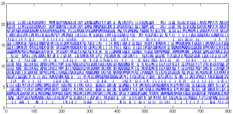
The second plot shows the output of all 800 small cells for each of 20 stimuli. This is the raw data entering the MDS caluclation. You can see the low amplitude stimuli are sparse (stimuli 1, 6, 11, 16). you can also see that the higher strength stimuli produce patterns which are similar within direction (e.g. 19, 20), but different between directions (e.g. 19,20 versus 14,15).

The third plot shows that the MDS analysis could find a reasonable 2-dimensional fit to the distance data, and that it make topological sense, because red is front positive, green is back positive, blue is left positive, and cyan is right positive. Only the lowest amplitude stimuli are not direction-resolved. Since fish come in different sizes (and thus amplitude), there is a basic ampliude/distance ambiguity. It seems to me that direction of approach is more important, and is clearly resolved.

The fourth plot shows that there is not much additional information gained by going to a 3-dimensional analysis. The four clumps are all abou the same distance above the floor. There may be some signal amplitude information in the vertical direction, however.

References

Bell CC and Grant K(1989), Corollary discharge inhibition and preservation of temporal information in a sensory nucleus of mormyrid electric fish, Journal of Neuroscience, Vol 9, 1029-1044,

Friedman MA, Hopkins CD (1998) Neural substrates for species recognition in the time-coding electrosensory pathway of mormyrid electric fish. Journal of Neuroscience 18:1171-1185.

Xu-Friedman MA, Hopkins CD (1999) Central mechanisms of temporal analysis in the knollenorgan pathway of mormyrid electric fish. Journal of Experimental Biology 202:1311-1318