T. Bartol; T. Sejnowski; B. Land; E. Salpeter ; M. Salpeter
(based on Neurosciences poster 422.17 presented at the Nov 2000 meeting)
Abstract
The simplest chemical kinetics scheme for the development of miniature endplate currents (mepcs) at the neuromuscular junction (NMJ) is:
To explain mepc characteristics (e.g. rise-time, amplitude, fall-time) with a simulation one has to assign numerical values to the four kinetics parameters, plus a diffusion constant (D) and quantal packet size. Previous measurements on lizard neuromuscular junctions (NMJ's) under various experimental conditions have led to one set of MCell simulation parameters (http://www.mcell.cnl.salk.edu) that match observed mepc characteristics. A major question of interest now is uniqueness of these simulation parameters and their relevance to other synapses. We carried out 47000 MCell simulations of a simplified NMJ to derive a table of 1568 sets of simulation parameters and their predicted mepc characteristics. With a slight loss of accuracy, only four parameters: b/a, b/k_, k+/k_ and D/k_ needed to be varied, allowing a wide range to be covered. The simulations were performed at the San Diego Supercomputer Center on BlueHorizon, an IBM SP with 1152 processors. The table is summarized in graphical form. An algorithm is presented for searching and interpolating the table for determining the range of simulation parameters which will equally well match mepc characteristics and for comparisons to other synapses. Supported by: NIH NS-09315 NSF IBN-9603611, and by NSF to the San Diego Supercomputer Center.
Glossary
Glossary nmj = neuromuscular junction
mepc = miniature endplate current
Physical input parameters:
Kp = forward binding constant (in 1/mol sec)
Km = unbinding constant (in 1/sec)
b = channel opening rate (in 1/sec)
a = channel closing rate (in 1/sec)
D = diffusion constant (in cm2/sec)
N = number of ACh molecules in a quantal packet (0.5N is maximum number of channel
openings)
h = height of the synaptic cleft (in microns) (bounded by two infinite planes)
s = density of ACh receptors (micron-2)
so = normal value of s
Three Timescales:
Binding time: tb = 1.39*h / (s *Kp)
Diffusion time for a 'saturated disk' of area (N/s):
td = 0.8*N / (4*p*s*D)
Mean burst duration for open channels: mbd = (1+b/2Km)
/ a
Three simulated conditions for mepcs (see also Fig 1 below):
(1) 'normal' : s = so
and acetylcholinesterase (AChE) intact.
(AChE parameters from Stiles, et.al. Biophys J. 77, 1177, 1999)
(2) 'noAChE': esterases omitted.
(3) 'reduced': s = 0.3*so
and esterases omitted.
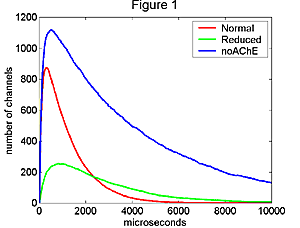 Figure 1. Simulated
mepcs under three conditions: (1) at normal AChR density, (2) with AChE removed
(3) with AChE removed and AChR density of 1/3 normal. All three were computed
using the same input parameters from the middle of the ranges described in the
Glossary
Figure 1. Simulated
mepcs under three conditions: (1) at normal AChR density, (2) with AChE removed
(3) with AChE removed and AChR density of 1/3 normal. All three were computed
using the same input parameters from the middle of the ranges described in the
Glossary
Output quantities from the mepc simulations:
tr = rise time (20% to 80% of peak during rising phase)
tf = fall time (90% to 33% of peak during falling phase) plateau time (80% during
rising to 90% of peak during falling phase)
P = plateau time / (tr tf ),0.5
hch = peak mepc amplitude,
expressed as number of open channels efficiency = (hch
/0.5N)x100 , expressed in percent (Measurement of rise time, fall time and plateau
are also shown in Fig 2).
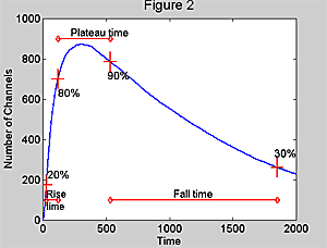 Figure 2. The measurement
scheme for simulated mepcs. Averaged traces were used in all cases. The peak
value was determined from a quadratic fit. Rise time, fall time, and plateau
time were measured as shown between the 20-80% rise, 90-30% fall and 80% rise-90%
fall respectively.
Figure 2. The measurement
scheme for simulated mepcs. Averaged traces were used in all cases. The peak
value was determined from a quadratic fit. Rise time, fall time, and plateau
time were measured as shown between the 20-80% rise, 90-30% fall and 80% rise-90%
fall respectively.
Experimental Target Values: Three dimensionless ratios predicted by Monte Carlo simulation results are:
(tr normal) / (tf normal)
(tf noAChE) / (tf normal)
(tr reduced) / (tr noAChE)
Experimental values of these ratios depend on the particular muscle and temperature,
but typical values are: tf normal ~= 1200 msec
tr normal ~= 90 msec
(tr normal) / (tf normal) ~= 13.3
(tf noAChE) / (tf normal) ~= 3.63
(tr reduced) / (tr noAChE) ~= 1.90.
MCell Simulations
Monte Carlo simulations of the reaction scheme outlined in the introduction were performed using MCell, a general simulation system for coupled reaction-diffusion systems with arbitrary bounding geometry. For the MCell simulations we fixed four quantities: h=0.05 microns, so=7500 AChR/micron2, N=5000 and mbd=1000 msec. These values imply tb=279/ Kp and td=212/D msec. We carried out 1568 sets of simulations separately for the three conditions 'normal', 'noAChE' and 'reduced'. These simulations covered all combinations of:
b/a = 100, 50, 20, 10;
b/2Km = 8, 4, 2, 1, 0.5, 0.25,
0.125;
tb = 279, 139, 70, 35, 17, 9, 4;
td = 200, 141, 100, 71, 50, 35, 25, 18;
To minimize stochastic noise, each set of simulation parameters was run 20 times and the results averaged. A quadratic curve fit was done near the peak to obtain an estimate of the amplitude. The estimated rise and fall times (Fig 2) were then obtained by line fits to appropriate portions of the mepc waveform. Each simulation set yields the output values tr, tf, hch, and P defined in the Glossary for each of the three conditions. The first version of the catalog (see below) consists of the input parameters and the corresponding outputs. The values of hch vary greatly and the values of tf vary slightly over the whole simulation catalog.
Some of the results are shown in Fig 3-5 below.
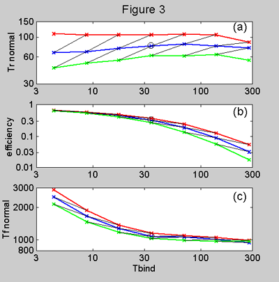 Figure 3. Model predictions
for (a) rise time, (b) efficiency, (c) fall time, plotted against binding time
tb. The simulations were for normal conditions with diffusion time td of 35
(green), 71 (blue) and 140 (red) msecs. In all cases b/a=50
and b/2Km=1. The thin,black
diagonal lines represent the effect of changing tb and td by the same ratio.
(a) Note that rise time varies remarkably little when tb is varied considerably
with td constant. Thus a pathological condition which increases cleft-height
h only, such as myasthenia gravis, would have little effect on the rising phase,
if s stayed the same. However, if td is increased
by dropping s (with BTX or a pathological condition)
then the rise time increases. (b) The efficiency decreases rapidly with increasing
tb, when tb is large. A disease which increases h/s
(such as myasthenia gravis) and thus decreases tb would have a less serious
effect on mepc amplitude if Kp were large. (c) For medium-to-large
tb, the fall time is close to the mean burst duration. Only for very small tb
is the binding to receptors so efficient that (even in the presence of esterase)
there is significant rebinding during the falling phase.
Figure 3. Model predictions
for (a) rise time, (b) efficiency, (c) fall time, plotted against binding time
tb. The simulations were for normal conditions with diffusion time td of 35
(green), 71 (blue) and 140 (red) msecs. In all cases b/a=50
and b/2Km=1. The thin,black
diagonal lines represent the effect of changing tb and td by the same ratio.
(a) Note that rise time varies remarkably little when tb is varied considerably
with td constant. Thus a pathological condition which increases cleft-height
h only, such as myasthenia gravis, would have little effect on the rising phase,
if s stayed the same. However, if td is increased
by dropping s (with BTX or a pathological condition)
then the rise time increases. (b) The efficiency decreases rapidly with increasing
tb, when tb is large. A disease which increases h/s
(such as myasthenia gravis) and thus decreases tb would have a less serious
effect on mepc amplitude if Kp were large. (c) For medium-to-large
tb, the fall time is close to the mean burst duration. Only for very small tb
is the binding to receptors so efficient that (even in the presence of esterase)
there is significant rebinding during the falling phase.
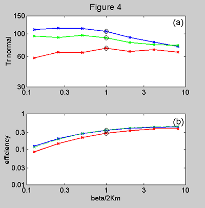 Figure 4. Model predictions
for (a) rise time and (b) efficiency plotted against b/2Km.
The plots are for values of the isomerization ratio b/a
of 10 (blue), 20 (green) and 100 (red). Note again that the rise time varies
very little with varying b/2Km,
especially for the most likely intermediate values of b/a.
The efficiency is somewhat small when b/2Km
is very small, i.e. when unbinding inhibits channel openings.
Figure 4. Model predictions
for (a) rise time and (b) efficiency plotted against b/2Km.
The plots are for values of the isomerization ratio b/a
of 10 (blue), 20 (green) and 100 (red). Note again that the rise time varies
very little with varying b/2Km,
especially for the most likely intermediate values of b/a.
The efficiency is somewhat small when b/2Km
is very small, i.e. when unbinding inhibits channel openings.
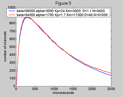 Figure 5. Two model
mepcs (normal condition) with different input parameters, but giving the same
values for tr and tf. The blue curve comes from a model with large Kp
and small D which gives a high efficiency of 54% while the red curve comes from
a model with small Kp and large D with quite low efficiency
of 6% (requiring a large N). The two mepcs are almost indistinguishable. The
shape of a mepc under normal conditions alone cannot give information on whether
the kinetics parameters lead to high or low efficiency. The ratio (tf noAChE)
/ (tf normal) is appreciably different for the two models, 51% for
the blue mepc and 5.6% for the red mepc. The relationship between this ratio
and the efficiency is shown in Figure 6.
Figure 5. Two model
mepcs (normal condition) with different input parameters, but giving the same
values for tr and tf. The blue curve comes from a model with large Kp
and small D which gives a high efficiency of 54% while the red curve comes from
a model with small Kp and large D with quite low efficiency
of 6% (requiring a large N). The two mepcs are almost indistinguishable. The
shape of a mepc under normal conditions alone cannot give information on whether
the kinetics parameters lead to high or low efficiency. The ratio (tf noAChE)
/ (tf normal) is appreciably different for the two models, 51% for
the blue mepc and 5.6% for the red mepc. The relationship between this ratio
and the efficiency is shown in Figure 6.
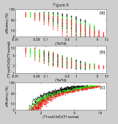 Figure 6. (a) A scatter
diagram of efficiency versus tb/td. Efficiency generally decreases as tb/td
increases, but as the color indicates, three ranges of tb+td are mixed together.
(b) A scatter diagram of (tf noAChE) / (tf normal) versus
tb/td. (c) A scatter diagram of efficiency versus the target ratio(tf noAChE)
/ (tf normal). The correlation between the two quantities is fairly
strong, since both decrease with increasing tb/td. The curvature is due to the
fact that (tf noAChE) / (tf normal) is always greater
than 1 and efficiency is always less than 100%. For all panels, the colors indicate
values for tb+td of >150 (red), 75 to 150 (green), and <75 (black).
Figure 6. (a) A scatter
diagram of efficiency versus tb/td. Efficiency generally decreases as tb/td
increases, but as the color indicates, three ranges of tb+td are mixed together.
(b) A scatter diagram of (tf noAChE) / (tf normal) versus
tb/td. (c) A scatter diagram of efficiency versus the target ratio(tf noAChE)
/ (tf normal). The correlation between the two quantities is fairly
strong, since both decrease with increasing tb/td. The curvature is due to the
fact that (tf noAChE) / (tf normal) is always greater
than 1 and efficiency is always less than 100%. For all panels, the colors indicate
values for tb+td of >150 (red), 75 to 150 (green), and <75 (black).
The Output Catalogs
Scaling Prescriptions
The six rate parameters plus the quantal packet size and diffusion constant of ACh are needed for a Monte Carlo simulation (see Glossary). There are two scaling arguments which greatly reduce the number of simulations required:
The model output must be converted from normalized, model units back to physical units for comparison with real data. If we start with an MCell simulation which produces some values for hch and tf (normal condition), we can convert to real units by defining two scaling factors: The amplitude scaling factor is defined as Sa=(actual amplitude)/(model amplitude) and the time scaling factor is defined as St=(actual falltime)/(model falltime). Multiplying the modeled waveform amplitude by Sa and the modeled waveform time by St scales the model waveform to the actual data. Removing the amplitude scaling for N and D consists of multiplying the model values by Sa. Removing the time scaling for a, b, Kp, Km, and D consists of multiplying by 1/St.
Range of Models which Fit the Three Target Values
Another version of the simulation catalog consists of the 1568 models which have been scaled so that all have amplitude hch=872 and fall time tf =1200 msec. With this scaling, the full range of parameter values explored by the models is; a =880 to 61000 1/sec, b=9100 to 2.7x10⁶ 1/sec, Kp=0.62 to 430x107 1/mol*sec, and Km=4900 to 4.9 x10⁵ 1/sec. Of the 1568 models, 73 predict all three target ratios (see Glossary) within 20%. Table 1a gives the range of kinetic parameters for this subset. With four input parameters to be chosen, and only three output quantities to fit to target values, we could not obtain input values uniquely. One therefore has to specify at least one input parameter (from experiment). For instance, many people have measured b although there seems to be a fairly wide range in reported values. In principle, by choosing some exact value for b and requiring an exact fit to three target values, there should be a unique set of reaction parameters. In practice, one has to accept an uncertainty range on each target value. The catalog user can specify the four uncertainty ranges and then obtain the set of models which satisfy the ranges. One example is in Table 1b and 1c. Two different ranges of b were chosen from the literature. Out of the 73 best fitting models, 9 have b within the range (60,000 to 100,000) shown in Table 1b, and 9 have b within the range (40,000 to 60,000) shown in Table 1c. Table 1b and 1c give the range of a, Kp, and Km for each range of b. If one specifies the value of a second input parameter to within some uncertainty range, the set of models is further narrowed. For instance, some measurements of a have also been done. If one specifies a to be in the range 2900 to 5000 (with b in the range in Table 1c), then only one of the 1568 models remaining is b/a=20, b/2Km=2, tb=70, td=100. On the other hand if one chooses a in the range 1500 to 2500, the only remaining model is b/a=20, b/2Km=1, tb=35, td=71.
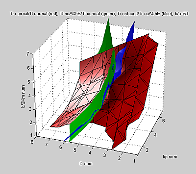
Another way of looking at the wide range of parameters which fit the data is
to plot surfaces representing the locus of parameters which yield each of the
three target ratios in input-parameter space. The following figure has axes
proportional to the logs of D, Kp, and b/2Km.
Since the green and blue surfaces (optimal
(tf noAChE) / (tf normal) and (tr reduced)
/ (tr noAChE) respectively) are almost conicident throughout the
parameter range, we lose power to uniquely fit data.
Conclusions