T. Bartol1; T. Sejnowski1; B. Land2; E. Salpeter2 ; M. Salpeter (deceased)
1. Salk Institute, La Jolla, CA, USA
2. Cornell University, Ithaca, NY, USA
(This page is based on poster 155.7 presented at the November 2001 Neurosciences meeting)
Abstract
One of the key issues in understanding synaptic transmission is the degree to which the number of neurotransmitter molecules in a quantal packet (Nn) saturates the number of receptors (Nr) on the postsynaptic membrane. In previous simulations of miniature postsynaptic currents (MPSCs) using MCell, a Monte Carlo simulator of subcellular signaling, we assumed that Nr >> Nn (see the MPSC catalog at http://www.mcell.cnl.salk.edu/database) which is appropriate for the neuromuscular junction (NMJ). Here we explore the range Nn >> Nr which is more appropriate for central synapses whose receptors are located within a small area.
One consequence of central synapse geometry and small Nr/Nn is that receptors
are saturated to a greater degree than at the NMJ (i.e. when Nr/Nn >>
1) and at the same time the current rise time is increased much less when the
receptor site density is reduced than at the NMJ. Measuring current rise times
after partial receptor inactivation may
thus yield information on Nr/Nn and degree of receptor saturation for some central
synapses. The diagnostic possibilities of the "plateau time", the
period separating the rising and falling phases of the MPSC, will also be presented.
All results are given in the form of dimensionless ratios, with special emphasis
on the ratio of fall time to rise time. MCell was run on BlueHorizon, a 1152
processor IBM SP supercomputer at the San Diego Supercomputer Center. The expanded
catalog is available at the above URL.
Supported by: NIH NS09315 (EES), NSF IBN-9985964 (TMB, TJS), and by NSF National Partnership for Advanced Computational Infrastructure at the San Diego Supercomputer Center.
Introduction
One of the key issues in understanding synaptic transmission is the degree to which the number of neurotransmitter molecules in a quantal packet (Nn) saturates the number of receptors (Nr) on the postsynaptic membrane. In previous simulations of miniature postsynaptic currents (MPSCs) using MCell, a Monte Carlo simulator of subcellular signaling, we assumed that Nr>>Nn which is appropriate for the neuromuscular junction (NMJ). Here we explore a range of Nn/Nr, which is more appropriate for central synapses whose receptors are located within a small area.
The major aim of the present work is to outline how the ratio ρ2=Nn/Nr affects the shape of the MPSC for fixed chemical kinetics parameters. We assume a slightly more general chemical model than in previous NMJ simulations by allowing cooperativity in two binding and unbinding steps. The general scheme is
where A2R and A2R* are the doubly bound closed and open channels, respectively.
Results will include:
(1) How MPSC risetime, falltime, and amplitude vary with ρ.
(2) Relation between lower receptor site density (perhaps by poisoning) and
increases in MPSC risetime. For the case when ρ>>1, as in the
NMJ, the increase is substantial, but for some models where ρ<1,
no increase was found.
(3) Previous work suggested that the MPSC plateau time (time near peak, expressed
in appropriate units) is surprisingly constant in the NMJ models when ρ>>1,
and we find this to be the case also when 0.1<ρ<10.
Modeling the MPSCs with Mcell There are more input parameters to this model than for the NMJ model we have used. There are six chemical-kinetic rate parameters, rather than the four without cooperativity. In addition to specifying the diffusion constant, D, the cleft height, h, the receptor density σ0, and the quantal packet size, Nn, we now have to specify the number of receptors, Nr, in the post-synaptic receptor disk. The receptor disk radius, Rr, and Nr are related by πσ0Rr,2=Nr. We define the "saturated disk radius", Rn, as πσ0Rn2=Nn and define the normalized receptor disk radius as ρ=Rr/Rn =(Nn/Nr)1/2. Our previous NMJ simulations had ρ>>1, but here we explore four separate cases with 0.1<ρ<10.
With seven input parameters we could afford only a small number of different values for each. For our main set of simulations we chose (and kept fixed) Nn=10,000 molecules; σ0=7,500 receptors/micron2; and h=0.028 micron. The diffusion constant, rate constants, and disk radius were varied through every combination of:
β/α = [1, 10]
β/2k-2 = [1, 10]
D = [2, 10]x10-6 cm2sec-1
k+2 = [1.4, 14]x107 M-1sec-1
k+1/k+2 = [0.1, 1, 10]
k-1/k-2 = [0.1, 1, 10]
ρ=[0.15, 0.61, 2.30, 7.67].
The unbinding rate constant, k-2, was specified by the observation that if there were no "buffered diffusion", then the falltime of the MPSC would equal the mean burst duration (MBD) which relates the chemical kinetics parameters as:
MBD=(1+β/2k-2)/α ---------- Eqn. 1
Instead of fixing k-2 we kept MBD=1000 msec. The number of parameter combinations computed was 2*2*2*2*3*3*4 = 576. Each case was repeated 20 times and averaged to reduce stochastic noise. The 20*576=11,520 Mcell runs were computed on BlueHorizon, a 1152 processor IBM SP supercomputer at the San Diego Supercomputer Center.
We also carried out simulations to explore the results of partial poisoning of the receptors by some toxin. We did this by setting &sigma=σ0/3 and repeating all 576 cases. Toxin was assumed to bind to ligand sites randomly so that 1/3 of receptors were functional but some ligand bound to receptors with one ligand site poisoned. There are two auxillary combinations of input parameters that have the dimensions of time:
tbind=1.39h/(σ k+2) ------------ Eqn. 2
tdiff=0.8Nn/(4π σ) ------------ Eqn. 3
The tbind is a measure of how long it would take for a agonist molecule to bind to a receptor if the receptor site density were uniform. The tdiff is a measure of how long it would take an agonist molecule to diffuse over a disk of &rho=1 in the absence of binding. We measure the rise time, tr, fall time, tf, as shown in Figure 1 below.
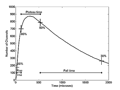
The plateau time is defined as the time between 80% on the rising phase and 90% on the falling phase, but we will use a normalized plateau time defined by:
P=(plateau time)/(tr tf)1/2 -------------- Eqn. 4
The MPSC amplitude (number of peak open channels, Nch) is also converted to two different efficiency measures: The efficiency in terms of the fraction of the quantal packet which is effective at the peak, queff=Nch/(0.5*Nn) and of the fraction of the number of receptors which are open at peak, raeff=Nch/(0.5*Nr). All of these outputs are cataloged and used for comparison to real MPSCs.
Results
Despite the large input ranges of various parameters (and their ratios), the variations in model output parameters (e.g. tf / tr) is generally surprising small. There tends to be a non-Gaussian distribution, with a clump of outputs and a few scattered outliers. Figure 2 shows tf / tr while varying k+2/k-2 for all the simulations with σ=σ0.
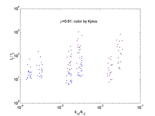
The points on the plot fall into six groups, but have been dithered horizontally to minimize overlapping points. From scaling considerations, we expected a strong positive correlation between tf / tr and k+2/k-2. The reasoning is that tbind is proportional to 1/k+2 and the risetime should be correlated with tbind. Similarly, the MBD is correlated with 1/k-2 and the falltime should be correlated with MBD. We therefore expected tf / tr to change strongly with k+2/k-2, which in Figure 2 varies over a range of 100. The actual results show only a very weak correlation, and perhaps even the wrong sign. The correlation seems to be weakened because smaller k+2/k-2 leads to lower efficiency, queff, which in turn leads to smaller risetimes, thus raising tf / tr.
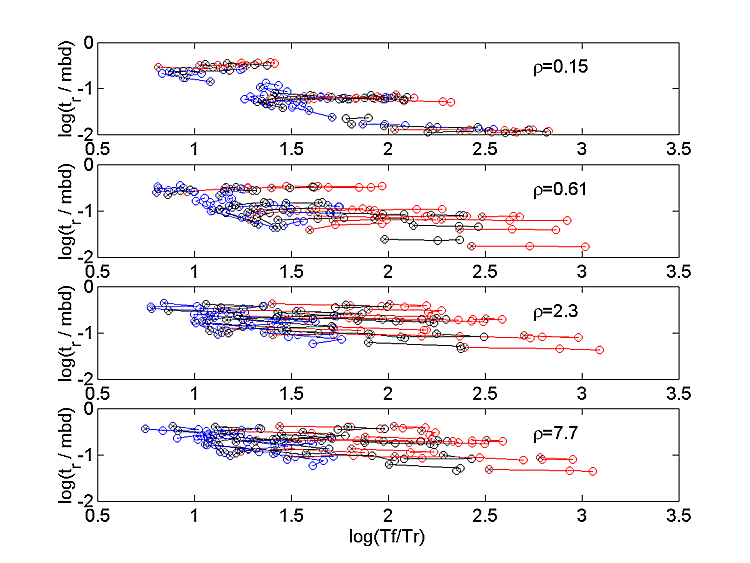
The simulated MPSCs yield efficiency and shape parameters for four different receptor patch sizes. The trends for tf versus queff and areff at each of the four ρ are shown in Figure 3 for all of the σ=σ0 simulations.
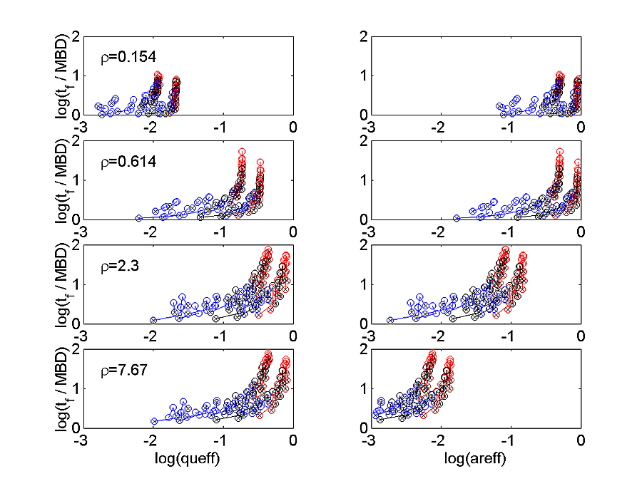
Each set of input parameters for which only k-1/k-2 changes is connected by a line. The end of the line with low k-1/k-2 is marked with an x. Each different k+1/k+2 has a different color with 0.1, 1, 10 colored as red, black, and blue respectively. The queff decreases as ρ is decreased, while areff actually increases. These effects make sense if most of the released agonist binds to available receptor. For small ρ, the receptors are used up before the agonist, so queff is low, but areff is high because almost every available receptor is bound. The tf also generally becomes smaller at small ρ. Figure 4 shows that tr also decreases with decreasing ρ, roughly in proportion to tf , so that tf / tr depends very little on ρ. The color and connection scheme is the same as for Figure 3.
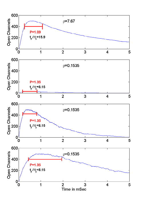
To compare the simulation results with actual data we have to remove the various scaling schemes that helped to reduce the dimensionality of the system. In our simulations, we varied the binding parameters k+2 and k+1/k+2, but fixed h. As long as the two radii Rr and Rn are large compared to h, only the ratio h/k+2 is important (for a given k+1/k+2 value). Hence of h and k+2 are multiplied by the same scaling factor (so that tbind stays the same), the results will stay approximately the same. Also, the fixing of the MBD (equation 1) represents a time scaling and fixing Nn represents an amplitude scaling. The model output must be converted from normalized, model units back to physical units for comparison with real data. If we start with an MCell simulation which produces some values for Nch and tf (normal condition), we can convert to real units by defining two scaling factors: The amplitude scaling factor is defined as Sa=(actual amplitude)/(model amplitude) and the time scaling factor is defined as St=(actual falltime)/(model falltime). Multiplying the modeled waveform amplitude by Sa and the modeled waveform time by St scales the model waveform to the actual data. Removing the amplitude scaling for N and D consists of multiplying the model values by Sa. Removing the time scaling for β, α, the four rate constants, and D consists of multiplying by 1/St.
One such example of such scaling is illustrated in Figure 5. Figure 5a shows a MPSC computed at large ρ. Figure 5b shows a MPSC computed at small ρ=0.15, but with the same kinetic parameters as in 5a. Figure 5c shows the small ρ MPSC with the amplitude scaling chosen so that the output amplitude equals the amplitude in Figure 5a. Figure 5d shows the same small ρ MPSC with both amplitude and time scaling chosen so that the fall time also equals that in Figure 5a.. Figure 5b shows that tr, tf, and Nch all decrease as ρ decreases.
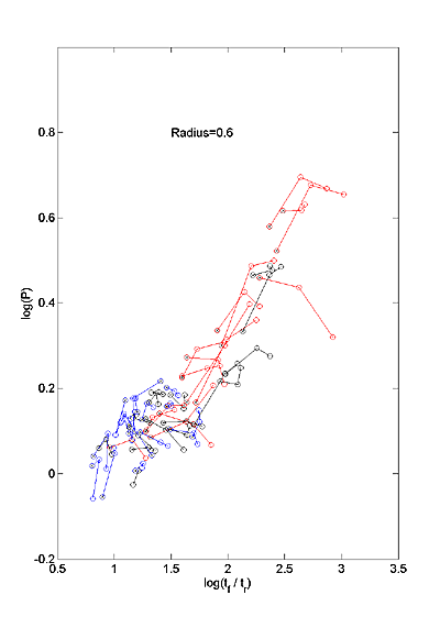
The normalized plateau time, P (equation 4), is a dimensionless shape parameter
that varies surprisingly little across parameter sets. Figure 6 is a scatter
plot of two dimensionless shape parameters, P versus tf / tr.
Colors and connections are as in Figure 3. P varies less than tf
/ tr. In the example shown with ρ=0.61,
P∼(tf / tr)s where s≅0.3.
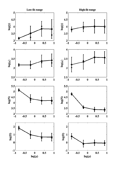
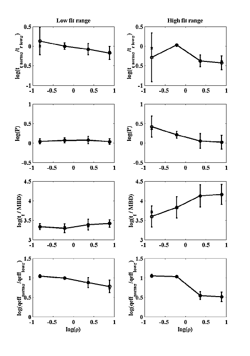
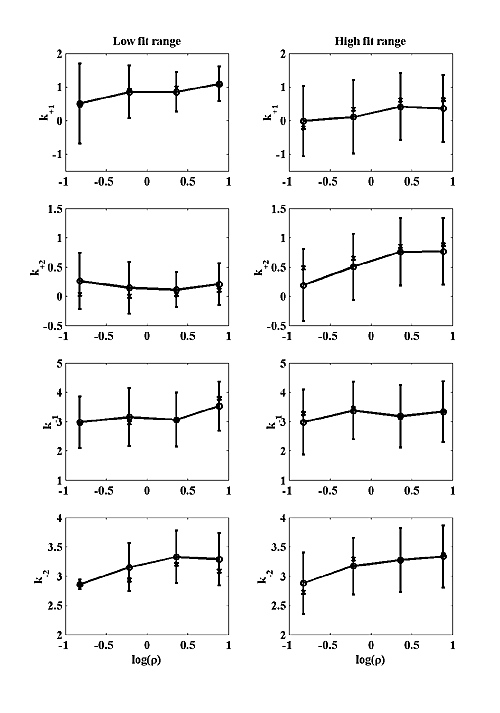
We attempted to fit our simulations to two hypothetical classes of MPSC that are not based on any actual data, but may be appropriate for some CNS synapse. We chose to fit only amplitude, fall time and tf / tr (at σ=σ0) because these parameters are the most likely to be available for real MPSCs. We picked a fairly small amplitude MPSC with 500 open channels at peak. Two fall times were chosen: 3 msec and 15 msec. For the 3 msec fall time we chose a log(tf / tr)=0.9±0.2 . For the 15 msec fall time we chose a log(tf / tr)=1.9±0.2 for the fit range. The chosen amplitude and fall time fix the model scaling parameters and the tf / tr becomes the single parameter that was matched to model output. All parameter values shown in Figure 7 have been converted back to real units by the process described above. The left column shows best fit parameters for the low fall time case and the right column for the high fall time case. The circles represent the averages of the log of each parameter, and are connected by a solid line. The error bars are the standard deviation of the log of each parameter. The x's represent the medians. Figure 7b shows that P is quite insensitive to model parameters in the low fit range and decreases perhaps a factor of two with increasing ρ in the high fit range. Figure 7b also shows that MPSC rise time does not necessarily increase with decreasing σ, which is different from the NMJ. For small ρ, the rise time is almost constant with decreased σ, but at larger ρ, the rise time dependency on σ is similar to the NMJ.
Conclusions
The simulations with 0.1<ρ<10 seem to share insensitivity of rise time and plateau time with the NMJ simulations we performed previously. Thus, there does not seem to be any shape parameter that will unambiguously resolve kinetic parameters from ρ for an unknown transmitter system under all regimes. On the other hand, if some synapse shows a plateau time appreciably different from the values in our simulations, it would indicate that a different model is required, perhaps one with slow exocytosis or a third ligand binding site.
Three values for used for each of k+1/k+2 and k-1/k-2. We checked the simulations which fell into the two fit ranges (described above) to see which values of the ratios predominated. The three ratios for k+1/k+2 gave about equally many fits, so that a restriction to k+1=k+2 does not seem to lose breadth of fit. The value of k-1/k-2, however, does effect the resulting value of tf / tr, especially at large ρ. For instance for ρ=7.67, none of the simulations which gave tf / tr between 5 and 12 (low fit range) came from k-1/k-2=0.1, whereas 15 of the 17 simulations came from k-1/k-2=10. Thus large values of k-1/k-2 are required for small values of tf / tr. For the high fit range (50<tf / tr<120) the situation is somewhat reversed. Only 2 of 27 simulations came from inputs with k-1/k-2=10. We conjecture that small values of k-1/k-2 may be required to produce very large values of tf / tr.
Acknowledgments
Supported by: NIH NS09315 (EES), NSF IBN-9985964 (TMB, TJS), and by NSF National Partnership for Advanced Computational Infrastructure at the San Diego Supercomputer Center.