Introduction
We needed to estimate a set of parameters and their errors for a nonlinear curve fit of cellular conductance data. The conductance was a function of voltage and was modeled as a Boltzmann term, an exponential term and a constant::
g = p3/(1+e((v-p1)/p2)) + p5*e((v-45)/p6) + p4
Where g and v are the input data, with v is in millivolts, and p1-p6 are the desired parameters.
A program was produced to:
The program
%Program for Matt Gruhn
%Written by Bruce Land, BRL4@cornell.edu
%May 20, 2004
%===================
%curve fit of 6 parameter conductance function of voltage
%Formula from Matt:
%g= (m3/((1+exp((m0-m1)/m2))^(1)))+(m4)+(m5*exp((m0-45)/m6));
%need to get parameters and their error range
%--Then separately plot the "boltzmann" and exponential parts separately
%===================
clear all
%total fit
figure(1)
clf
%part fit
figure(2)
clf
%parameter histograms
figure(3)
clf
%========================================================
%START settable inputs
%========================================================
%data set 1 from Matt-- cell f
%the voltages
x=[-30.3896
-25.2314
-20.0655
-14.9218
-9.82205
-4.71594
0.380856
5.53925
10.749
15.8878
21.0423
26.154
31.3026
36.3964
41.4244
46.3951
];
%the measured conductances
y=[0.01428535
0.032721504
0.06306213
0.099658404
0.134567811
0.162306115
0.181366575
0.196532089
0.20765796
0.218294045
0.22529785
0.235617098
0.250215255
0.268659046
0.294750456
0.331398216
];
%estimate of error in conductance measurement
%Currently set to 2%
dy = y*0.02;
%formula converted to
%The inline version
func = inline('p(3)./(1+exp((x-p(1))/p(2))) + p(5)*exp((x-45)/p(6)) + p(4)','p','x');
%initial parameter guess
p0 = [-10 -7 -0.2 -.01 0.2 8 ];
%To detect the sensitivity of the fit to starting parameter guess,
%the fit is run a number of times.
%each fit is plotted and each parameter plotted as a histogram
Nrepeat=100;
%each parameter is varied by a normal distribution with
%mean equal to the starting guess and std.dev. equal to
%sd*mean
sd = 0.3;
%histogram zoom factor (how many std dev to show)
zfactor = 2;
%parameter outlier cuttoff: lowest and highest N estimates are removed
outcut=10;
%========================================================
%END settable inputs
%========================================================
%list of all parameter outputs to use in histogram
pList=zeros(Nrepeat,6);
for rep =1:Nrepeat
rep
%form the new randomized start vector
p = [p0(1)*(1+sd*randn), p0(2)*(1+sd*randn), p0(3)*(1+sd*randn),...
p0(4)*(1+sd*randn), p0(5)*(1+sd*randn), p0(6)*(1+sd*randn)];
%do the fit
[p,r,j] = nlinfit(x,y,func,p);
%copy fit to list
pList(rep,:) = p';
%get parameter errors
c95 = nlparci(p,r,j);
%conductance errors
[yp, ci] = nlpredci(func,x,p,r,j);
%plot the fit
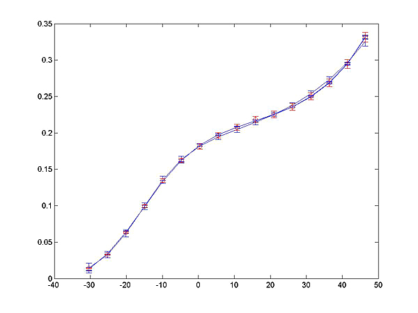
figure(1)
errorbar(x,func(p,x),ci,ci,'b-');
hold on
errorbar(x,y,dy,dy,'ro')
%plot the separated fits
figure(2)
subplot(2,1,1)
hold on
errorbar(x, y-func(p,x)+ p(5)*exp((x-45)/p(6)),dy,dy,'rx')
%plot(x, (y-func(p,x)+ p(5)*exp((x-45)/p(6))),'ro')
errorbar(x, p(5)*exp((x-45)/p(6)), 2*ci, 2*ci,'bx-')
title('Exponential fit')
subplot(2,1,2)
hold on
%plot(x, (y-func(p,x)+ p(3)./(1+exp((x-p(1))/p(2)))),'ro')
errorbar(x, y-func(p,x)+ p(3)./(1+exp((x-p(1))/p(2))),dy,dy,'rx')
errorbar(x, p(3)./(1+exp((x-p(1))/p(2))), 2*ci, 2*ci,'bx-')
title('Boltzmann fit')
%drawnow
end
figure(3)
%plot and print parameter table
fprintf('\r\rFit parameters and 95percent confidence range\r')
for i=1:6
subplot(6,1,i)
lowerLimit = mean(pList(:,i))-zfactor*std(pList(:,i));
upperLimit = mean(pList(:,i))+zfactor*std(pList(:,i));
hist(pList(:,i),linspace(lowerLimit,upperLimit,30))
%
fprintf('%7.3f\t +/- %7.3f \r',...
mean(pList(:,i)),...
max(2*std(pList(:,i)),mean(pList(:,i))-c95(i,1)));
end
fprintf('\r\rFit parameters omitting outliers\r')
for i=1:6
%get rid of outliers
pup = sort(pList(:,i));
pup = pup(outcut:end-outcut);
%print again
fprintf('%7.3f\t +/- %7.3f \r',...
mean(pup),...
max(2*std(pup),mean(pup)-c95(i,1)));
pbest(i)=mean(pup);
end
%print conductance table
%based on best parameters
v = [-30:5:45];
clear yp ci
[yp,ci] = nlpredci(func,x,pbest,r,j);
fprintf('\rVolt \t Total g\t Boltz\t Exp \r')
for i=1:length(v)
fprintf('%7.3f\t%7.3f\t%7.3f\t%7.3f\r',...
v(i),...
yp(i),...
pbest(3)./(1+exp((v(i)-pbest(1))/pbest(2))),...
pbest(5)*exp((v(i)-45)/pbest(6)));
end
Typical output
There is graphical and text output from this program. Each figure represents 100 curve fits to the same data. The first figure is a plot of the total curve fit, while figure 2 are the components of the curve fit. Figure 3 are the histograms of 100 different fits to the same data. Also shown are the raw (all sets) parameter means and the the selected (removing outliers). Note the outliers in each figure, and the strong central tendency of the parameter estimates. Finally the program prints a table of voltages and the fit values of total conductance, Boltzmann part, and exponential part.
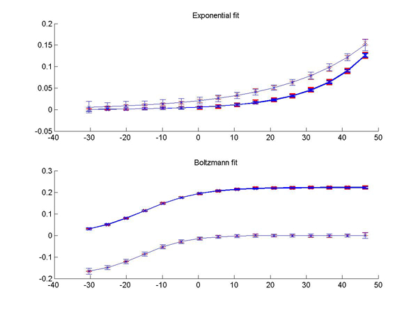
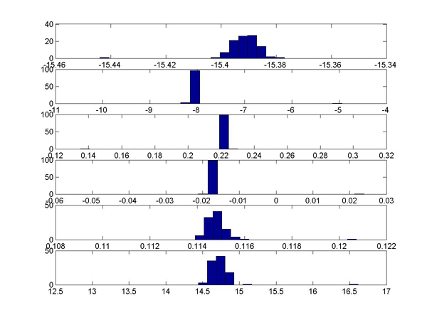
Fit parameters and 95percent confidence range
-15.394	+/-   0.611
 -7.951	+/-   1.457
  0.219	+/-   0.041
 -0.016	+/-   0.019
  0.115	+/-   0.006
 14.805	+/-   1.461


Fit parameters omitting outliers
-15.391	+/-   0.614
 -8.098	+/-   0.583
  0.223	+/-   0.014
 -0.018	+/-   0.008
  0.115	+/-   0.006
 14.713	+/-   1.370

 Volt    Total g  Boltz   Exp
-30.000	  0.013	  0.032	  0.001
-25.000	  0.034	  0.052	  0.001
-20.000	  0.064	  0.081	  0.001
-15.000	  0.099	  0.114	  0.002
-10.000	  0.133	  0.147	  0.003
 -5.000	  0.162	  0.175	  0.004
  0.000	  0.183	  0.194	  0.005
  5.000	  0.197	  0.206	  0.008
 10.000	  0.208	  0.214	  0.011
 15.000	  0.217	  0.218	  0.015
 20.000	  0.225	  0.220	  0.021
 25.000	  0.236	  0.222	  0.029
 30.000	  0.250	  0.222	  0.041
 35.000	  0.269	  0.223	  0.058
 40.000	  0.295	  0.223	  0.082
 45.000	  0.331	  0.223	  0.115
Revision to eliminate constant term
The fit equation was modified to
g = p3/(1+e((v-p1)/p2)) + p4*e((v-45)/p5)
which eliminates the constant term. For some parameter sets, particularly where the total curvature of the data is small, the constant term tended to make the fit unstable. The convergence criteria were more carefully monitored to make sure that the overall fit was reasonable.
Reference
Gruhn M, Guckenheimer J, Land BR , Harris-Warrick R (2005)
Dopamine modulation of two delayed rectifier potassium currents in a small neural network, Journal of Neurophysiology, 94: 2888-2900 (pdf)