Introduction
We needed a specialized program to help automate the collection of spike train data and reduction to ISI histograms and other formats. The input data was contaminated with large stimulus artifacts, but the signal to noise ratio was generally good. Since the stimulus artifacts did not overlap actual motor nerve spikes we could null the artifacts by gating the signal based on the stimulus monitor.
The basis for the program was the Matlab DAQ toolbox and assosicated file format. Data was collected using a virtual oscilloscope and logged directly to disk with time stamps. Channel one carried the spike train, while channel two carried the stimulus monitor.
The program source is here for version 22.
Program description
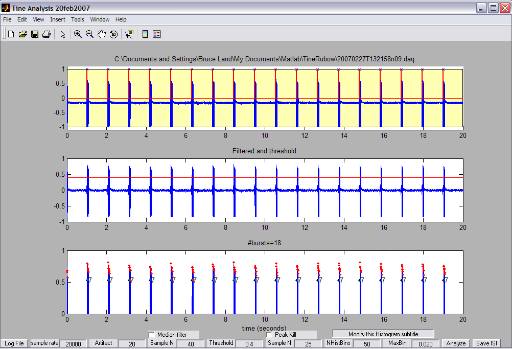
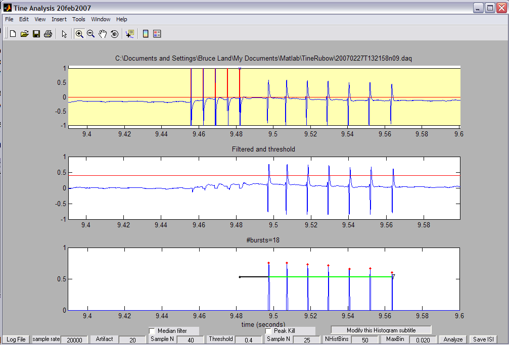
The image below (which can be expanded) shows the interface. The three panels show:
The output window shows a ISI histogram.
 The histogram shows the bins in the region of interest. The top title is the file name being analysed. The subtitle title is a string entered from an edit field in the main window and the portion of the file which was selected in the main window (corresponding to the pale yellow region in panel one above).
Control Description
The controls are:
Log File button: This button opens a dialog box to pick a daq file type with two channels. The program assumes that channel one carries the spike train and channel 2 the stimulus monitor unless you check the box. Sample rate: This edit field must match the value used in the data aquisition program. Default is 20,000 samples/sec. This value is autoset by the daq file and the control is disabled.Artifact: This edit field chooses how many samples to force to the mean after each stimulus. Default is 20. Setting this control to zero disables the artifact cancellation.Median filter: This checkbox and edit field enables and sets the length of the median filter. The filter length should be set to be somewhat longer than the spike duration, but numbers above 50 samples may take a long time to filter. Threshold: This edit field sets the voltage level for spike analysis. It can be positive or negative depending on which phase seems the cleanest.Peak kill: This checkbox and edit field enables and sets the length of the region in which two or more peaks will be collapsed into one peak. The peak chosen is the biggest (or smallest of a negative threshold is set).NhistBins: This edit field sets the number of bins used in the output figure.MaxBin: This edit field sets thetime range of bins used in the output figure.Analyse button: Takes all the inputs and computes results.Save ISI button: Writes a textfile with burst statistics and the interspike intervals in it. The data file name and other information are also written. The numbers are comma-delimited for ease of import into spreadsheets.Output file format
An example output file is shown for two bursts in the middle of the train shown above. The header material shows the data file name, an optional subtitle, and the time interval actually used for analysis. Each burst is listed, along with averages. A complete list of ISIs (with the sequence number with the burst) is included for further analysis. The zeros in the sequence list are the interburst ISIs.
  C:\Documents and Settings\Bruce Land\My Documents\Matlab\TineRubow\20070227T132158n09.daq
Modify this Histogram subtitle
Analysis region=5.638710 to 8.967742 sec

burst#, latency, duration, spike#
   1,  0.01713,  0.06665,    7
   2,  0.01548,  0.06630,    7
   3,  0.01538,  0.06625,    7

#bursts, latency,  STD,    duration,  STD,    spike#,  STD
   3,  0.00380,  0.00568,  0.06640,  0.00022, 56.00000, 29.14063

List of all ISIs in the region
0.009750, 1
0.011150, 2
0.011150, 3
0.011100, 4
0.011350, 5
0.012150, 6
0.990550, 0
0.009800, 1
0.011200, 2
0.011300, 3
0.011050, 4
0.011300, 5
0.011650, 6
0.992300, 0
0.009800, 1
0.011250, 2
0.011200, 3
0.011150, 4
0.011200, 5
0.011650, 6