Introduction
Neurons use sterotyped, pulsed signals called action potentials to signal over long distances. Since the shape of the action potential is believed to carry minimal information, the time of arrival of the action potential carries all the information. Often the detailed voltage waveform is abstracted into a stream of binary events where most of the stream represents no action potential occurence ('zeros') and an isolated '1' represents an action potential. The binary waveform is refered to as a spike train.
The current talk is focussed on temporal coding in spike trains. It seems to me that temporal coding, as used in neurobiology, refers to any time code, including a pure rate code as a special case. One can think of many examples:
Since spike trains are sending messages to synapes (typically), it might be useful to ask how we can interpert a spike train in a way which makes synaptic sense. A first approximation might ask: Over what time scale does the synapse integrate information? If the integration time is very short, then only events which are close together matter, so synchrony in a code is a useful concept. On the other hand, if integration time is long, then the total number of spikes matters, so a rate code is a useful concept. Perhaps we should analyse spike trains on every time scale. In addition to time scale, we could analyse trains in several ways, each corresponding to a different (measured, or hyopthesized) aspect of synaptic function. For instance activation and learning might have different effective coding from the same spike train.
We want to talk about schemes for finding patterns in spike trains, Bruce will descibe patterns in EOD discharge data and I will describe some theoretical techniques which seem to hold promise in their flexibility and potential synaptocentric (love those neologisms) orientation. The thread between them is the use of methods that avoid some problems with traditional binning methods. Specifically, we will consider schemes that treat the spike time as the most important variable.
Techniques
Spike train analysis is the attempt to find patterns in spike trains which reflect some aspect of neural functioning. This could include
There are many techniques for understanding a temporal code, for instance:
The techniques we will explore here are based on reference (1), (2)and (3). These avoid problems with binning in time and allow the flexibility of imposing synaptic interpretations on the train. Bruce has talked about how convolving a train with an Gaussian distribution allows a smoother, more relable estimate of burst parameters. What we want to do now is describe how spike trains might be compared to each other for similarity.
To set the stage, let us consider a pure rate code. Each train is then specified by its rate, and the difference between trains is the difference of their rates. We could say the the distance separating the trains is the difference of their rates, or that rate differnce is a distance measure between spike trains. What we would like is a distance measure which works on any time scale. Then we could speak of the distance between two trains with a given time precision. Such a distance measure would allow us to smoothly go from strict synchronization codes (very small spike time difference allowed) to rate codes (large time differences allowed within an overall interval). The time resolution at which you analyse the train might alsocorrespond to the time constant of the synapse.
Two recent papers describe techniques for computing the distance between two spike trains at any time resolution. Victor's paper (1) define the distance between two spike trains in terms of the minimum cost of transforming one train into another. Only three transforming operations are allowed; move a spike, add a spike, or delete a spike. The cost of addition or deletion is set at one. The cost of moving a spike by a small time is a parameter which sets the time scale of the analysis. If the cost of motion is very small then you can slide a spike anywhere but it still costs to insert or delete a spike, so the distance between two trains is just the difference in number of spikes. This is similar to a rate code distance. If the cost of motion is very high then any spike is a different spike,so the minimum costs become the cost insert or delete all the spikes. The distance between two trains becomes approximately the number of spikes in the train which are not exactly alligned, sort of a measure of synchrony. Intermediate values of cost interpolate smoothly between perfect synchrony and a rate code.
Rossum's paper (2) computes a distance which is closely related to Victor's distance, but much easier to implement and easier to explain. Each spike train is convolved with an exponential function:
e(-(t-ti)/tc) with t>tiWhere ti is the time of occurence of the ith spike. You get to choose the time constant tc of the exponential, which sets the time scale of the distance measurment. Call the convolved waveforms f(t) and g(t). You then form the distance as:
D(tc) = (dt/tc) * sum[ (f(t) - g(t))2 ]
Where dt is the spike sampling time step. This distance could
be considered as an approximate differnce between two post-synaptic current
sequences triggered by the respective spike trains because such currents tend
to have approximately exponential shape. In a sense, the Rossum distance measures
the difference in the effect of the two trains on their respective synapses
(to a very crude approximation).
The Rossum time scale, tc, and Victor's cost parameter are related by
cost = 1/tc
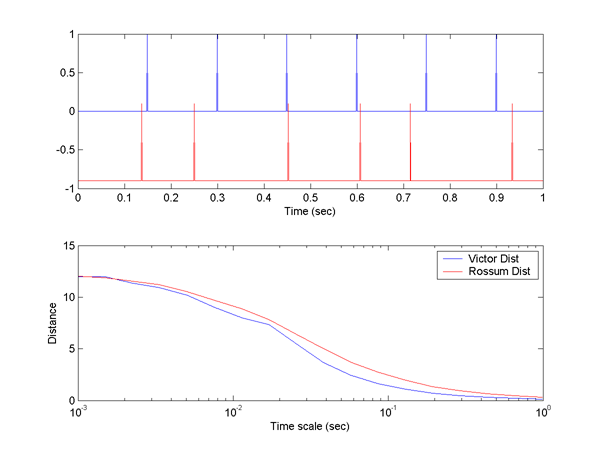
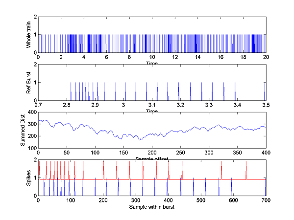
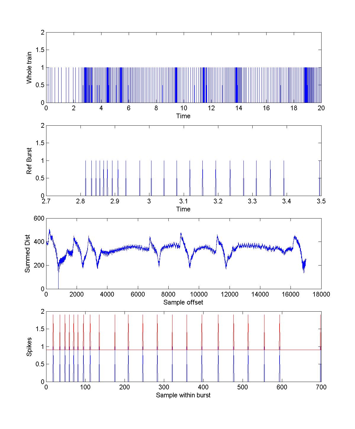
We can compare the two distance measures over a wide range of time scales using this reciprocal relation. Two of the matlab programs given below do this comparison, but an example here might help. The following image shows two spike trains. The blue train is regular and the red train is a gaussian dithered verson of the blue train. At small time scales, the Victor distance is 8 because 4 spikes are not exactly aligned. This means that 4 spike deletions and 4 insertions are necessary to transform one into the other. At time scales comparable to the dither (in this case std.dev.=10 mSec), the Victor distance starts to drop because it is cheaper to move a spike. At long time scales the Victor distance goes to zero because both trains have the same number of spikes. The Rossum distance falls more smoothly because it depends on a smooth exponential weighting function. The distance at short time scales is similar because the exponentials have essentially fallen to zero. At large time scales the Rossum distance also goes to zero, because it too measures the total number of spikes. Which distance you decide to use depends on how you think the spike train is interpreted post-synaptically. Note that the distance is computed at all possible time scales so that different criteria of synchrony are automatically available.
Once we can compute distances between spike trains, we can try out several techniques outlined in reference (1). The following assumes that trains are caused by some controlled stimulus, and can therefore be a-priori catagorized by the stimulus type. These steps have been implemented in the software described below.
Uses of a spike train distance measure:
Code
Matlab distance programs. To run the following programs, you will need to download the routine spkd from Cornell Med.
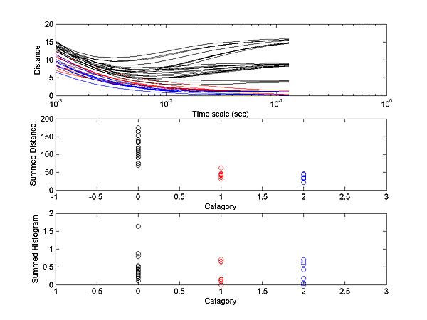
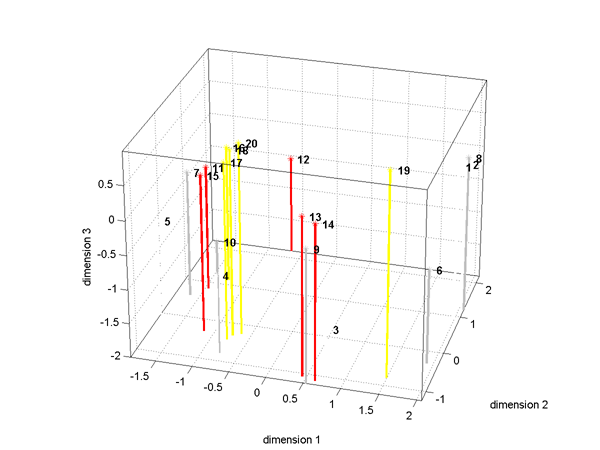
fminu must be modified to call fminunc.The fist image shows the optimal imbedding of the train
distances in 3D (data from previous image). The numbers correspond to individual
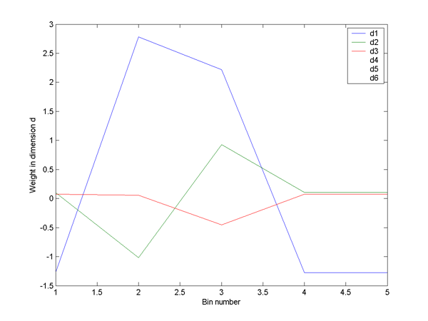
trains and the colors to the 4 groups. The second image is the temporal profile
for this 3-space using 5 time-bins for each spike train. It shows that dimension
1 is coding a weighted sum so that high values aling the axis mean a low initial
firing rate, then a high rate, followed again by a low rate. The second dimension
is encoding a temporal pattern of approximately the first derivitive of dimension
1. 
Tools on the Web.
References
Copyright Cornell University, 2003