Oscilloscope using a microcontroller and a TV

Introduction

I wanted to see if I could make a useful scope using just a microcontroller and a television. The result works, but is a bit slow with a maximum sampling rate of 15,750 Hz. This is fast enough for most electrophysiology, but not for audio. The sampling rate is determined by the maximum rate of the internal A/D converter.

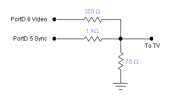
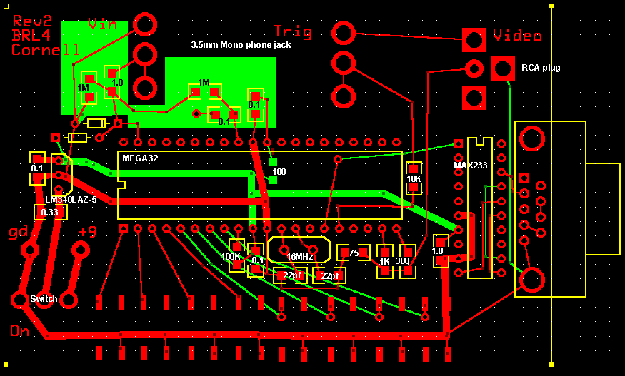
The entire scope consists of a Mega32 microcontroller, 8 push buttons (connected to one port), and a TV. Optionally, you can add an RS232 interface to dump waveforms to a computer. The DAC to connect the microcontroller to the TV is shown below.

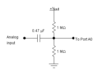
The analog input to the scope consists of a 0.47 microfarad capacitor and two 1.0 megaohm resistors as shown below. The highpass cutoff is around 1 Hz. The two resistors bias the A/D input to Vref/2. The capacitor blocks DC from the input. Input must be limited to +/-2.5 volts.

The full schematic:

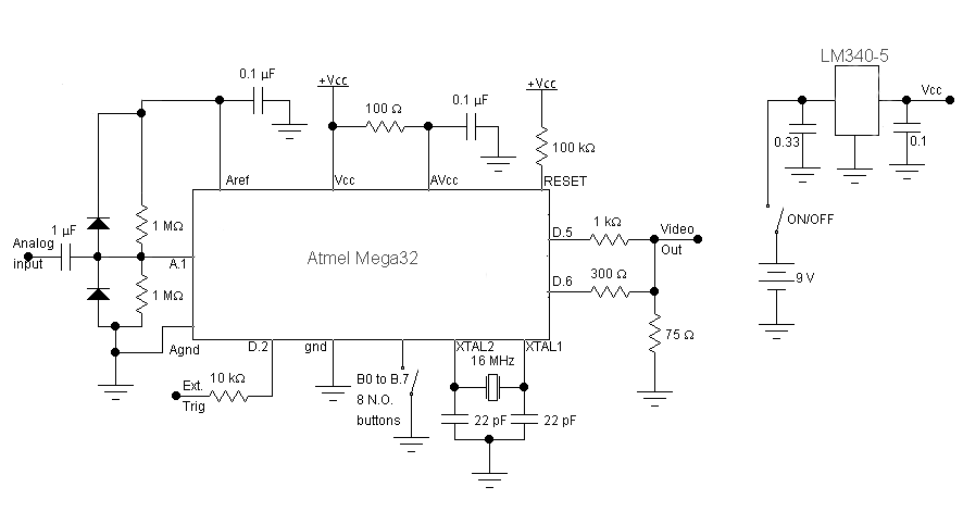
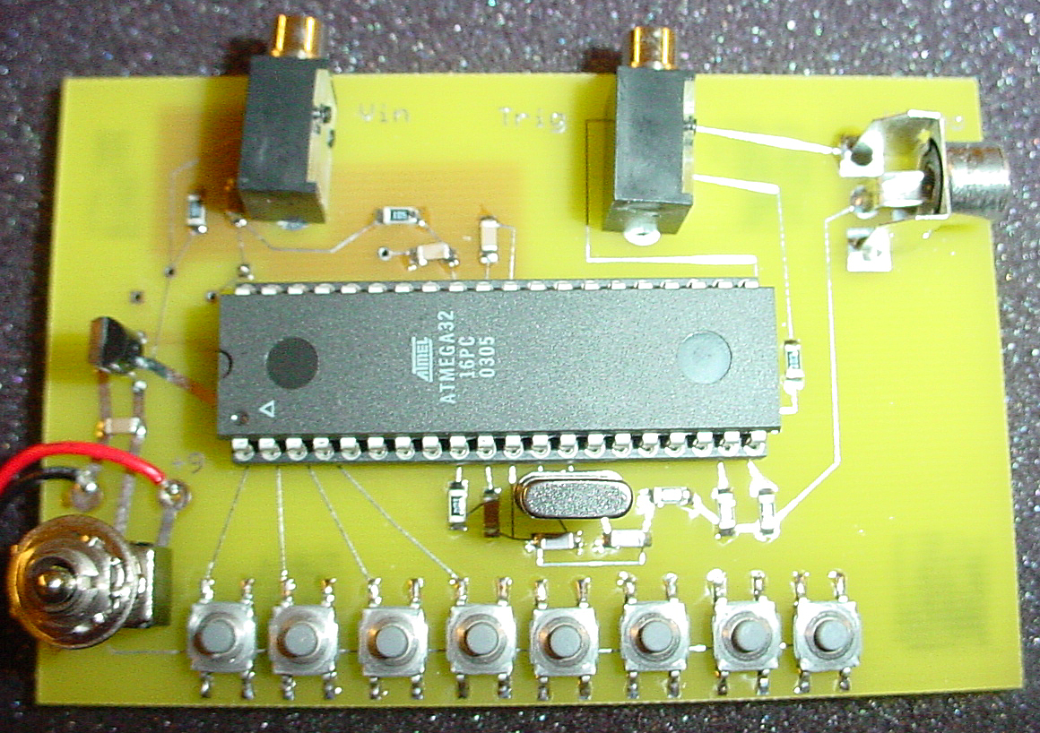
The external trigger input is just a logic level directly into the INT0 input which is PORTD.2. The system runs on a 16 MHz crystal at 5 volts.The curcuit board is shown below (version 1 without RS232). The ExpressPCB (do a save as... on the following link and use ExpressPCB software) design file is for the version with RS232 output.

Parts list (Digikey part numbers):

• MEGA32-16PC Atmel microcontroller
• MAX233ACPP dual RS232 interface.
• A2100 RS232 connector socket
• LM340LAZ-5.0 regulator
• 901K snap-fit phone jack, 90-degree
• CP-3502N mono 3.5 mm audio connector socket
• 401-1103-1 rubber surface-mount push puttons
• CTX077 16 MHz crystal
• All resistors and capacitors are 1206 surface-mount packages

Scope details

Scope freatures:

• Displays one voltage channel.
• Full scale voltage range of 5, 2.5, 1.25 and 0.75 volts.
• Full scale time range of 8, 16, 33, 65, 130, 261, 521, 1042 mSec.
• Samples at 15.75 kHz maximum (NTSC video line rate).
• Cursor measurement of time and voltage on the trace.
• Calculation of RMS voltage of the trace.
• Trigger on edge/level, with settable value. External logic-level trigger.
• RUN/STOP modes with single trace capture.
• Waveform dump to the UART.

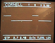
The CodeVision C program is loaded on the Atmel Mega32. The above image shows two pulses. The dot just below the trace is the cursor. Below that there is a RUN/STP/ARM indicator, cursor readout of time and voltage on the trace, a LEVL/EDGE/EXTN/FREE trigger indicator, and the trigger level. The current time and voltage scales are shown in the upper right corner.

Buttons:

• Button 0 toggles RUN/ STOP mode.
• Button 1 arms a capture in STOP mode. The capture actually occurs when the trigger condition is met.
• Button 2 cycles the trigger mode to LEVEL/EDGE/EXTERNAL/FREERUN.
• Button 3 changes the time scale in RUN mode. The time scale cycles through eight values.
  
• Button 4 changes the voltage scale in RUN mode. The voltage scale cycles through four values.
• Button 5 dumps the waveform to the serial port in STOP mode. The video is stopped during the dump. See example below. Button 5 computes the RMS voltage value of the trace in RUN mode.
  
• Button 6 decrements the trigger level in RUN mode. It increments the cursor position in STOP mode.
• Button 7 increments the trigger level in RUN mode. It decrements the cursor position in STOP mode.

Internally, the program is divided into two parts:

• The timer1 compare-match ISR runs at video line rate. The ISR:
  • generates the horizontal and vertical synch pulses
  • blasts bits from RAM to the video output
  • checks for a trigger condition, and acquires a voltage sample, if the time is right.
  • An external trigger pulse is latched by the INT0 interrrupt flag, but there is no associated ISR, rather the timer1 ISR poles and clears the flag.
• The main program:
  • Sets up the environment, draws some strings, and drops into the usual endless loop
  • the loop sleeps until the whole video screen is drawn by the ISR, then during the vertical sync time:
    • draws a new trace, if it ready
    • runs the button debounce state machine
    • performs the button actions (move cursor, draw strings, etc) and sets flags for the ISR

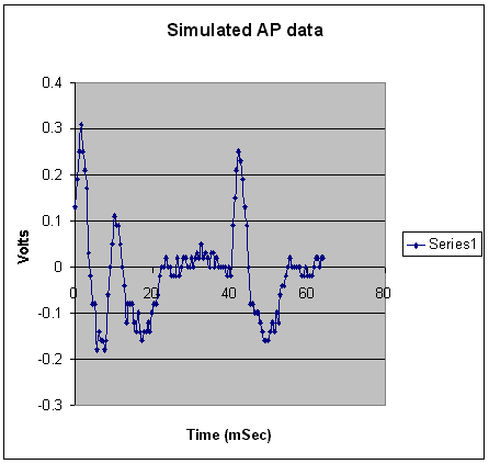
The serial port dump allows analysis of individual traces. A trace dump to a PC and then plotted by Excel is shown below. The actual data shown is simulated AP data fed into the scope from the sound port of a PC.

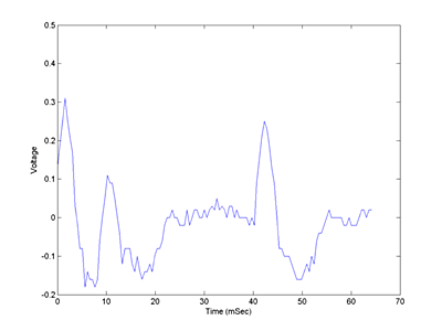
The Matlab commands

clear all
load 'a:\dump1.txt' -ascii
plot(dump1(:,1),dump1(:,2))
xlabel('Time (mSec)')
ylabel('Voltage')

produced the plot below:

Copyright 2003 - Cornell University