Introduction
We wanted to investigate the relationship between action potentials occuring in the motor nerve controlling vocal production in the plainfin midshipman and action potentials occuring in the auditory nerve. The relationship could have implecations for gain control of the ear during vocalization.
The process
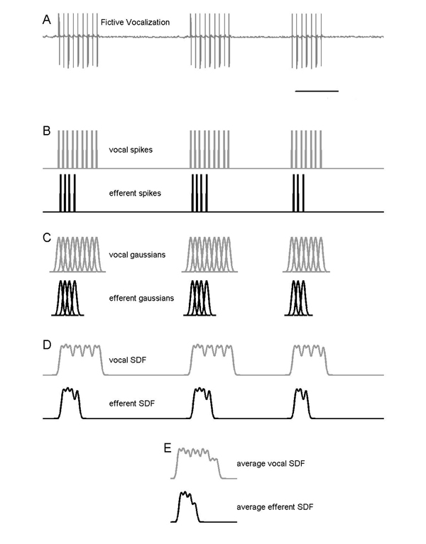
When vocally active sites within the midbrain were stumulated with glutamate, motor neurons produced a series of fictive grunts. Simultaneous recording from the auditory nerve often showed correlated efferent activity. Recordings could include as many as 70 fictive grunts from each motor neuron, and associated auditory nerve efferent activity. To ensure unbiased interpretation and to automate data analysis, we designed a procedure to produce an average vocalization spike activity and a synchronized average efferent activity. To do this we needed to align the start (or end) of each vocalization. Then we averaged spikes across all the aligned vocalizations. the begining (or end) time of the vocalization was used as a reference to align the efferent activity for each fictive grunt.
We tried several schemes to accomplish the alignment. First we tried using the first spike in a fictive vocalization as a trigger for a 'post trigger histogram'. this did not produce satisfactory results be cause the narrow bin width necessary to resolve the temporal structure caused excessave aliasing (due to bin edge effects). We settled on a spike density function (SDF) scheme because we could control the degree of smoothing and because the Gaussian we used as the SDF kernel is very good at reducing aliasing. The following figure shows the process we used. The data shown in the figure is typical of data we recorded, but is synthesized calibration data.
The steps in the process:
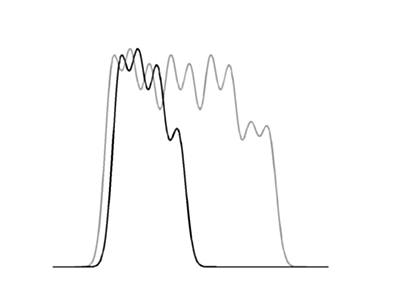
Expanding the time scale of E above and overlaping the traces, you can see below that the time of average occurance of efferent spikes are shifted in time relative to the vocal spikes. In this example, the efferent spikes were just shifted copies of the vocal spikes and were all shifted the same amount in order to check the averaging algorithm. The shift was equal to 1/2 of the first vocal ISI. The real efferent data shows a more interesting pattern of phase-locking.
The programs
All programming was done in Matlab 6.5 from the Mathworks. The program does the following operations:
vocwidth = 5;
voctk = -3*vocwidth:3*vocwidth ;
vockernel = exp(-(voctk/vocwidth).^2/2)/(vocwidth*sqrt(2*pi));
Reference:
Weeg MS, Land BR, Bass AH (2005) Vocal Pathways Modulate Efferent Neurons to the Inner Ear and Lateral Line, Journal of Neuroscience, June 22, 2005, 25(25):5967–5974 (pdf)
Copyright Cornell University, 2004