"A data logger & visualization platform for extreme sports enthusiasts."
project soundbyte
The idea of the project was to create a useful and commercial product for winter sport enthusiasts. We both love skiing so we wanted a product that could provide us with information and a way to visualize our skiing behaviors. The initial idea that we wanted to create was a skiing HUD with responsive voice feedback. We quickly realized that this project would not be reasonable with the time constraints that we had. However the motivation behind the project remained the same. We therefore decided on the idea of a data logging device that could be paired with a MicroSD card and a python script to visualize and track progress of skiing runs throughout your day.

High Level Design top
Overview
The motivation behind this project is that it involves skiing, an activity that we both love doing. In addition, sport technology is becoming increasingly popular with commercial products such as the GoPro and certain other extreme 'smart' sport optics, helmets, and FitBits that give the user added abilities and pertinent information. The rise of this type of technology is due to two factors. The first is an increase in the amount of information that we share on social media. Having the ability to track and share where you ran, your latest scuba diving experience, or your ski run down Corbet's Coulier in Jackson Hole gives the user something to tell his friends about and actually show them what it was like. This gives the user positive reinforcement and motivation to keep doing the things he or she loves. The second factor is for safety and convenience. Many of these activities such as riding a motorcycle, skiing a double black diamond, or diving 100 meters underwater involve many risks that if solely under the user's control would impede the ability to perform and have fun. In an effort to make such activities safer, the point is to provide the user or athlete with as much real time information as possible to allow them to make the smartest decisions possible in the shortest amount of time. As we shifted toward a focus on a data logger rather than an actual HUD, we shifted our focus to providing feedback that can be stored on a MicroSD card to the user rather than using real time data.
The device recieves data from an accelerometer, a gyroscope, and a temperature and pressure sensor in order to create a snapshot view of a user's local acceleration, velocity, temperature, and altitude. This data is then logged to a MicroSD card where the user can run a python script on the csv file saved in the MicroSD directory in order to create data that can be plotted using Microsoft Excel or MATLAB. The data received from the accelerometer is in an analog voltage format for x,y, and z directions. The data received from the pressure sensor includes temperature in degrees Celsius, pressure in Pascals, and altitude in meters. The data received from the gyroscope includes x,y, and z axis rotation rates in degrees per second.
In order to generate a useful output for the user to analyze, the data that we log from the accelerometer and gyroscope need to be corrected to compensate for gravity.
Accelerometer & Gyroscope Theory - Compensating for Gravity
Accelerometer's can be visualized as a ball inside a cube. With no gravitation fields or any force on the ball, the ball would simply float in the middle of the box as shown below. This is the case if for example, the box were far in outer-space. If we suddenly move the box to the left with an acceleration equal to 1g, the ball will hit the wall "X-". The pressure force that the ball exerts on the wall is measured and output as a value on the positive X-axis.
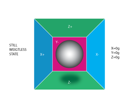
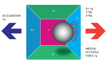
Left: Accelerometer in Weightless State. Right: Accelerometer accelerating to the left.
If we know consider the accelerometer as being on the Earth's surface. Now, the force of gravity is pulling down on all objects at a constant 1g=9.8m/s^2. In this case, the gravitation force pulls the ball down inside the cube so that it hits the -Z wall. This would produce a -1g reading on the Z-axis. Up to this point, we have simply considered one dimensional problems along one axis at a time, however that is not the case when the accelerometer and the device is in motion. Now, the force can be spread out over two walls or axes or even possibly 3 axes. If we rotate the box that we've been using, 45 degrees to the right, the force of gravity now has components along both the -Z and -X axes. The angle of rotation determines the components along each axes as the cosine of the angle. Now the problem has essentially become a question of the projections onto the 3- orthogonal X,Y, and Z axes of the gravitational force vector. If we are able to know the angle, then we can compensate for gravity.
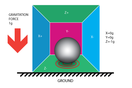
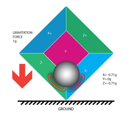
Left: Accelerometer on Earth's surface Right: Accelerometer on Earth tilted 45 degrees to the right.
The solution involves the gyroscope, gyroscopes can measure the rotation around one of the axes. For a triple axis gyroscope like the one we used for our project, this measures the angular velocity around the X,Y, and Z axes. By combining the Pythagoream Theorem to the accelerometer values and updating our calculations with the gyroscope measurements, we were able to create our own IMU or inertial measurement unit.
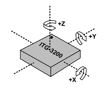
Gyro and axes of rotation.
Logical Structure of Program
Pseudocode:
SetupADC();

			CalibrateAccelerometer();

			InitializeSPI2();

			InitializePressureSensor();

			InitializeGyro();

			while (!FSInit()); //if card is detected and formatted correctly

			while (1) {

				   ax, ay, az = readAccel();

				   gx, gy, gz = readGyro();

				   temp, pressure, altitude = readPressure();

				   WriteDatatoSD(ax, ay, az, temp, pressure, altitude, gx, gy, gz);

			}
Block Diagram
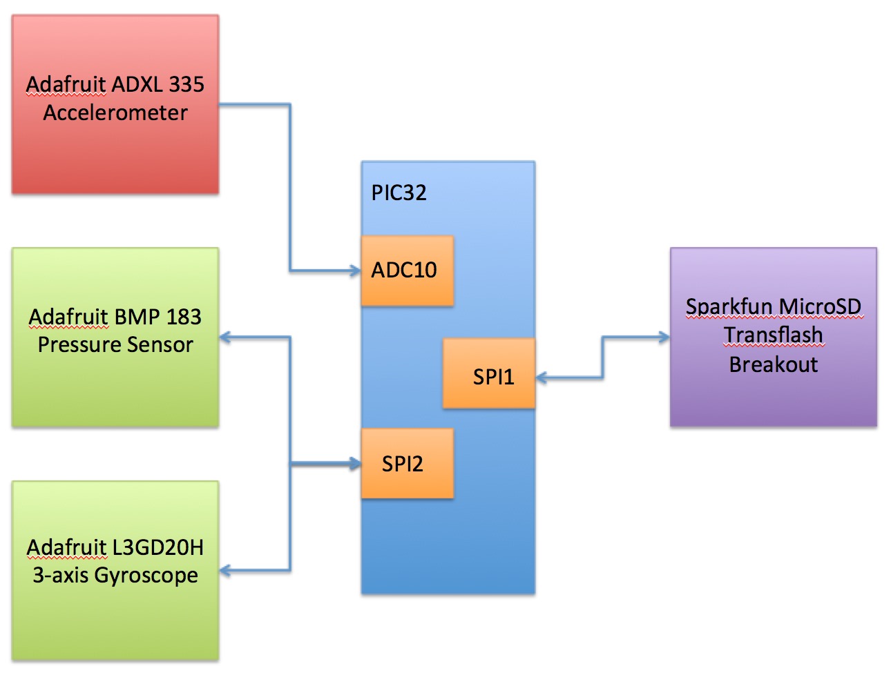
Hardware and Software Tradeoffs
There were several tradeoffs for the hardware and software used in the project. First, in software, because we were limited to using a single core processor in the PIC32, we were limited in the synchronization of our data. The protothreads that we used to implement our data logging and collection are not actually multi-threaded so data collection for the accelerometer occurred at a different time than data collection from the gyroscope. This made it very difficult to accurately compensate for gravity and led us to estimate by linear interpolation the time synchronization of these data sets. Additionally, we wanted data collection to occur as fast as possible for certain functions like the accelerometer and gyroscope because we knew that this data would be changing at a much faster rate than data from the pressure and temperature sensor. Thus, we updated the temperature, pressure, and altitude data about every second whereas the gyro and accelerometer were calculated about ten times per second.
For hardware, we tried to minimize the complexity of our peripherals. We decided to use SPI or Serial Peripheral Interface in order to communicate with the gyro, pressure sensor, and SD Card. This enabled us to use the same clock (SCK2) and data lines (SDI/SDO) for calculating the pressure and gyroscope values. Additionally, we would have liked to put all of our sensors and PIC32 on a solderboard in order to make a compact device and then have some sort of case over the circuitry and sensors to protect them from getting wet or snowed on while skiing. However, due to time constraints, this package was left out. In the end, we believe that this would be necessary if this were to become a fully- functioning device that had applications in cold, harsh environments.
Standards
SPI
To communicate between the microcontroller and the different sensors, the 4-wire SPI protocol was used. The microcontroller served as the single master for all of the slave sensors. The CS or chip select is the serial port enable pin and is controlled by the SPI master, in this case the PIC32 microcontroller. This pin is configured as an output and goes low at the start of data transmission for a specific slave and then goes back high in the end. The SPC or SCK is the serial port clock and is also controlled by the SPI master. The clock frequency can be as fast as the peripheral bus clock configured at 40MHz, but generally is much slower due to thresholds and maximum data rates of certain slave devices. SDI and SDO are respectively the Serial Port Data Input and Output. The PIC32 supports two SPI channels that can be configured with unique clock frequencies and data lines. The SPI2 channel shared clock (SCK2) and data lines, MISO (Master-In-Slave-Out) and MOSI (Master-Out-Slave-In), but had different chip select (CS) lines in order to run the pressure sensor and gyroscope off the same SPI Bus. The MicroSD breakout ran exclusively with the SPI1 channel. All of the SPI channels were initialized in Master mode, with 8 bits per char, clock edge reversed, and an SPI frequency of 2MHz.
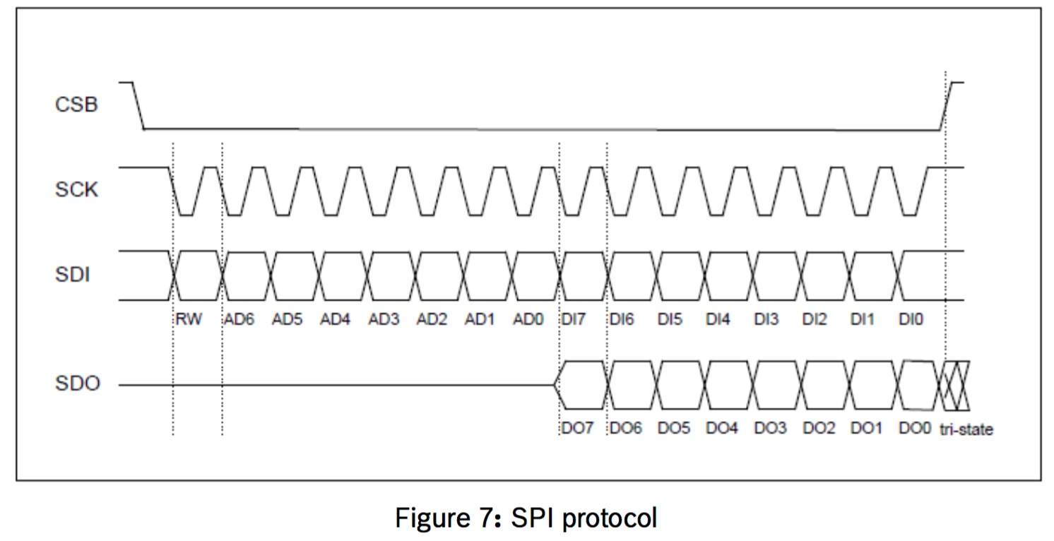
4-wire SPI Protocol
FAT32
In order to communicate and write with the MicroSD card, we conformed to the FAT32 file structure on most SD Cards today. In addition, this file structure was supported in the MDD Microchip Libraries for Applications that we ended up using for our communication protocol with the breakout board.
Existing Work
Even before we executed our project, there is a product on the market that inspired some of the functionality of our original intended device. A company called Recon Instruments makes a device called the Snow2 which they describe as the "next generation GPS Heads-up Display for Alpine Sports." Clearly, our project doesn't use a GPS to track a user's motion, however we do include many of the on-board sensors that they use including a gyroscope, accelerometer, and barometer.
Additionally, we found a similar Cornell ECE 4760 project done in the Fall of 2014 by Jason and Jeff Setter that used a GPS system to navigate and track through Google Maps waypoints. Although our project is considerably different in our approach and the different sensors being used, the idea to track and report data was a similar aspect especially with regard to winter sports such as skiing.
Hardware top
Hardware Design
TODO: Total Circuit Diagram
Accelerometer and Gyroscope - Inertial Measurement Unit
The accelerometer and gyroscope sensors provide the core data behind the user's relative motion. The accelerometer that we used was the Adafruit ADXL 335. This particular sensor output analog voltages for all 3-axis: X, Y,Z. These analog voltages were read into the microcontroller using the built-in ADC10. The x-direction corresponded to analog pin 4 (AN4) or physical pin 6. The y-direction corresponded to analog pin 5 (AN5) or physical pin 7. The z- direction corresponded to analog pin 11 (AN11) or physical pin 24. This enabled us to gather acceleration data and mapped it to a range from 0-1024 corresponding to a voltage from 0 (Low) to 3.3 (High). In order to find the acceleration due to gravity, we tried to measure the force of gravity along each axis. This required initial calibration in order to average out the accelerometer's measurements and also closely correlate the accelerometer data with the gyroscope. The Gyroscope that we used was also from Adafruit. The specific device that we used was the L3GD20H, a MEMS motion sensor three-axis digital output gyroscope. We used this device to gather data about rotation about all of the 3-axis in units of DPS (degrees per second). We retrieved data from this sensor using the SPI2 channel with the standard 4-wire SPI protocol that we mentioned above. It is extremely important to note that the serial data out (SDO) pin from the microcontroller connected to the serial data in (SDI) pin on the slave devices, in this case the gyroscope. The clock line was the standard PIC32 SCK2 or physical pin 26. The data out (MOSI) line we chose to be RPA4 or physical pin 12 while the data in line (MISO) we chose to be RPA2 or physical pin 9 on the microcontroller. The chip select for the gyroscope was RPB5 or physical pin 14. The combination of the accelerometer and the gyroscope formed our attempt at synthesizing our own inertial measurement unit.
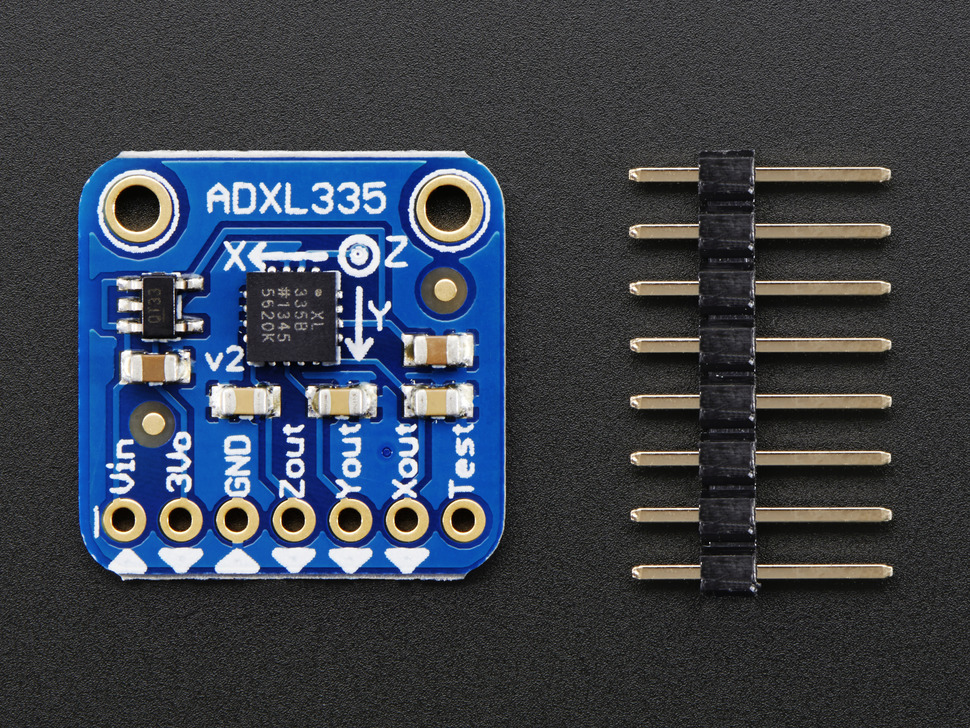
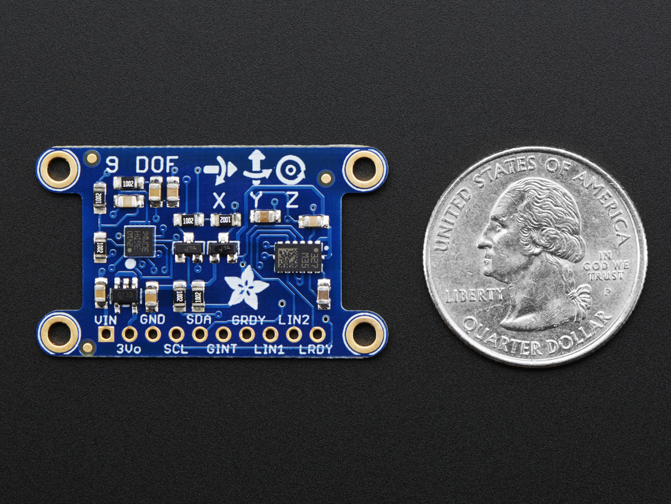
Left: ADXL335 Accelerometer. Right: L3GD20H 3-axis Gyro.
Pressure Sensor
Pressure and temperature were one of the first things that we wanted to implement and existed from the original project idea. By having an accurate measure of these statistics, we knew we could accurately show accurate altitude changes as well as weather shifts during a ski run down a mountain. This could also help us analyze our vertical displacement rate or downward velocity. The pressure sensor that we used was the Adafruit BMP 183. This sensor we also communicated with via SPI channel2. As we mentioned earlier, this sensor shared the SPI channel with the gyroscope, but this didn't matter because both had unique chip select pins. The chip select pin for the pressure sensor was RPB7 or physical pin 16. The pressure sensor outputted temperature and pressure data which we then used to calculate altitude. The BMP183 was designed to be connected directly to a microcontroller by the SPI bus. The pressure and temperature data had to be compensated with built-in calibration unique to each device. This "E^2PROM" data was initialized before data acquisition to properly calculate the pressure and temperature from the raw inputs. This specific device consisted of a piezo-resistive sensor, an analog to digital converter and a control unit with the calibration data registers and an SPI interface.
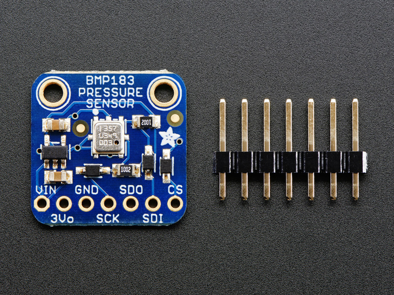
BMP183 Pressure Sensor
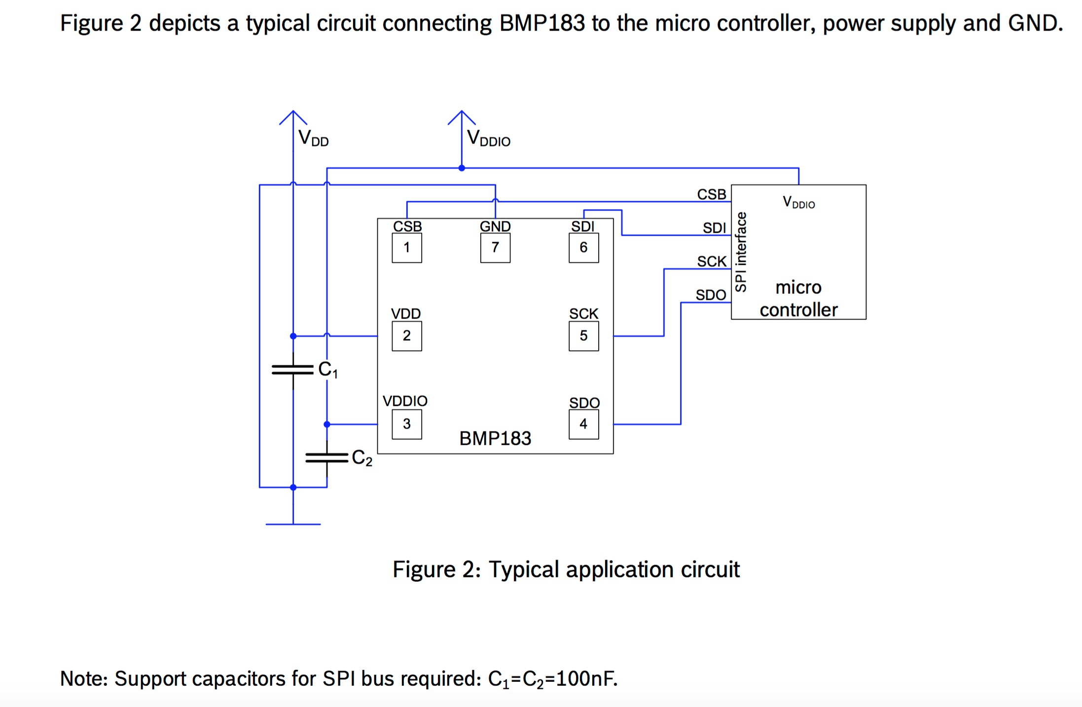
Circuit with the PIC32.
MicroSD Transflash Breakout
The idea of incorporating an external memory space was not in the intial plans for our project. However, as we shifted over to a logger device, we knew that a MicroSD would be perfect to save and log performance data for later analysis. In order to communicate with the MicroSD card and store our data, we needed a breakout board. The one that we used was from Sparkfun. We decided against using the MicroSD on the TFT because we wanted to save money and also eliminate the display because we wanted the device to be discrete and also for safety reasons for possible distractions when you are skiing or doing active outdoor sports. The MicroSD breakout ran using the SPI1 channel and used the following pins: SCK1 (pin 25) was the clock, RPB9 (pin 18) was the CS, RPB11(pin 22) was the MOSI, RPB8 (pin 17) was the MISO, and finally RPB10 (pin 21) was the CD or chip detect. The chip detect pin would check whether or not a MicroSD was inserted into the card holder. All of the sensors described above were connected to a common power and ground that came off the Vdd and Gnd pins of the microcontroller.
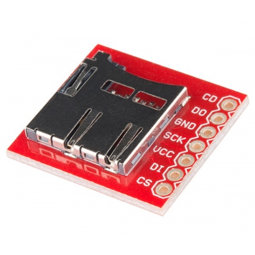
MicroSD Transflash Breakout from Sparkfun
LCD Debugging - Not included in final project
Throughout the process of building and debugging our device, we relied heavily on the TFT LCD to debug the particular sensors that we used. However, in the end we decided to remove the TFT from the project because it would not serve a purpose in data logging and only increased the computing overhead and also for safety considerations discussed later.
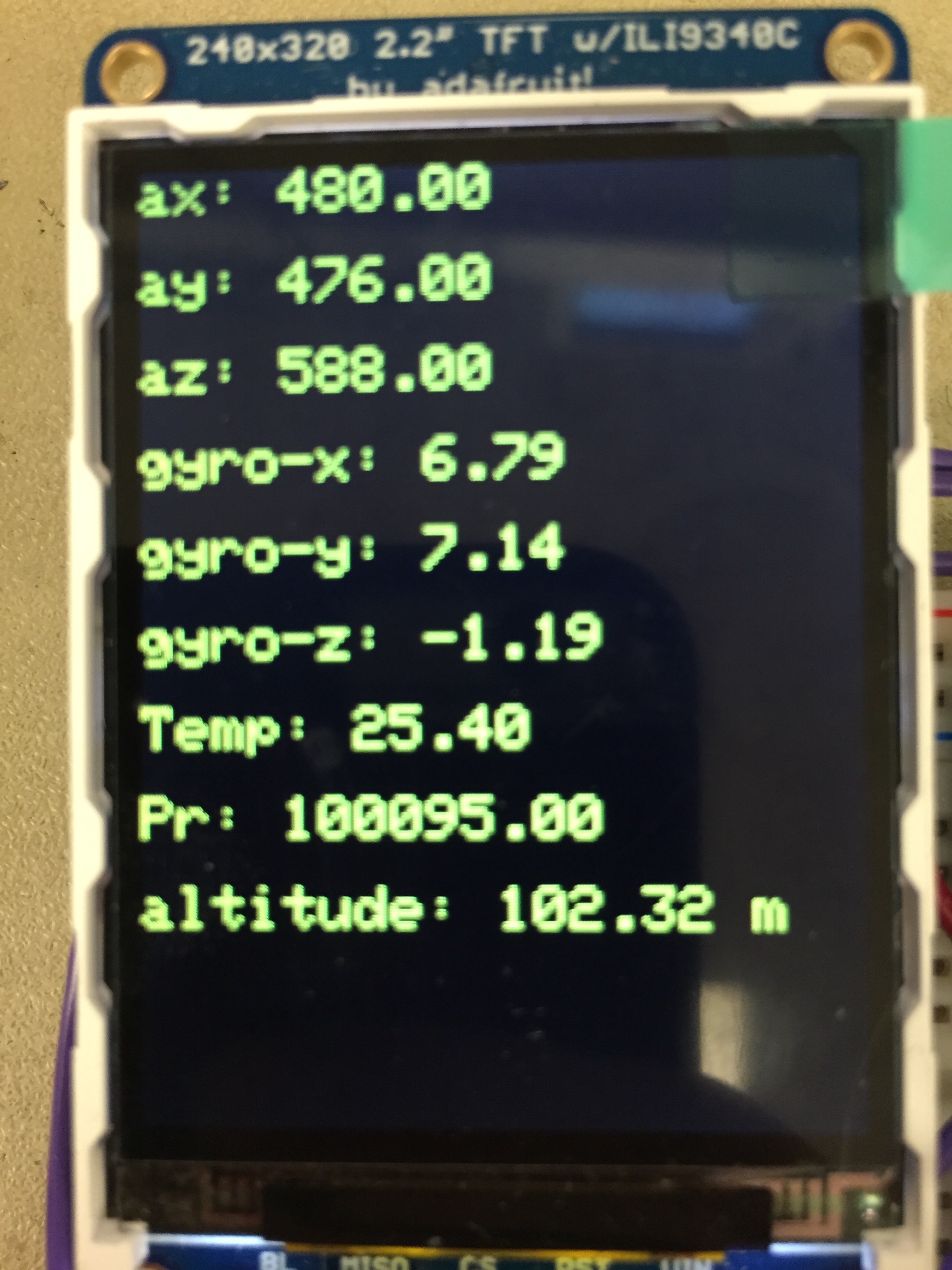
Screenshot of TFT LCD Display during a Debugging Run showing unadjusted accelerometer, gyroscope, pressure, temperature, and altitude data.
Software top
PIC32 Software Overview
The software for this lab was written entirely in the C programming language in the MPLABX IDE. Just as in the previous laboratories in the ECE 4760 class, the protothreads library was utilized to get data from all the different sensors and log data onto the microSD card. Four protothread structures were used for each specific function. One to toggle the ADC and get acceleration data, another to retrieve the temperature, pressure, and altitude data, another to get the gyroscope readings for each axis, and finally one to save the most current data to the microSD card in a ".csv" file format. The specific functions and complementary files are discussed next.
Analog to Digital Conversion
In order to read the analog inputs from the accelerometer sensor, we had to set up and use the built-in analog
to digital converter, ADC10. We wanted to output in integer values between 0 and 1023 and chose to enable
autosampling. we used the peripheral bus clock (PBClock). Additionally, we set the three analog input pins that we
were using to measure the x,y, and z vectors of acceleration. In our main function, we opened and enabled the
ADC10 module. We then used the Protothreads library provided from "pt_cornell_1_2.h" in order to have a separate
acceleration thread that simply measured each value sequentially. In the thread, we first set the channel using the
function SetChanADC10() to the first analog input pin, AN4 that corresponded to the x-direction of
acceleration. We then yielded the thread for 2 milliseconds to allow for the channel to be set correctly. Next, we read
the value of the analog pin using the function ReadADC10() and set the value to the corresponding
static variable. The last piece of the code that we used was a microsecond timer for more precise time measurements
in order to integrate the acceleration to find the velocity. This was achieved through a Timer2 interrupt that
incremented a variable time_microsec every microsecond. This integration proved to produce large
accumulating errors in often varying functions as we will explain later, so this technique was abandoned in favor of
post-processing numerical integration in the python script.
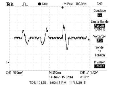
Y(bot)AccelwithoutLPF.jpg)
Left: X-axis acceleration analog input. Right: X(top) and Y(bottom)-axis
acceleration analog inputs.
Please right click and open images in new tab for better viewing.
The above graphs show the analog input voltages from the X and Y data out lines from the accelerometer during a test movement. The first graph on the left shows just the X-axis acceleration. As we can see, steady state no movement produces a fairly noisy signal. We tried to correct for this with a simple passive low pass filter, but it did not produce a significant improvement. The positive edge spikes correspond to an acceleration in the positive x-axis direction, while the following negative spikes correspond to decelerating by the same amount. This makes sense because we tested them by quickly snapping them in one direction with our hands and then stopping so the acceleration to produce the initial snap was then immediately followed by a deceleration to stop the movement. In addition, it is important to note that orthogonal axis were fairly well isolated from each other. This is shown from the X and Y axis outputs from the graph on the right.
As we can also see from the screenshots above, the value of the x-axis accelerometer analog input was about 1.5-1.6V which is a little smaller than half of the reference 3.3V. This means that for any axis orthogonal to the gravity vector, the analog reading of the accelerometer should fall right in the middle of the low and high reference voltages. It clearly wasn't exactly 1.65V for each axis so we had to research and calibrate each axis separately. Since the acceleration of gravity is a constant, we could use it to calibrate our respective 3-axis sensitivity. We did this by measuring the effect of the acceleration of gravity on each axis to find what the output analog voltage was for +/-1g or +/-9.8m/s^2. This proved helpful in extrapolating our acceleration values to correct units in the post processing stage.
TO-DO: talk about analog to digital converters and the scale that we used from 0-1023
SPI Data communication
The spi data communication between the microcontroller and the various sensors was essentially the foundation of data collection for our project. Each sensor, the pressure and the gyroscope as well as the sd card breakout had a different spi protocol. The majority of the lab was focused on building the integration of software for communicating with each of these external boards by SPI.
Pressure Sensor
The first board we worked with was the Adafruit BMP183 pressure sensor. This sensor came with plenty of
documentation on how to setup and receive data. Because we had both the pressure sensor as well as the gyroscope
communicating by the SPI2 channel, we first initialized the channel in the main function before beginning any
pressure calibrations. The SPI channel was configured to run at 2MHz because this produced the least noisy clock
and data waveforms to ensure accurate data (both devices had a maximum clock frequency of 10MHz). All of the
SPI functionality for the pressure sensor was written in the corresponding header and source files:
pressure.h and pressure.c. The header file initializes all of the registers that we
communicate with. The 16-bit register addresses of calibration data start from address 0xAA and go to address 0xBF.
We also initialize the Mode Settings that the sensor will be running in. This mode setting is passed as an input to the
pressure_begin(unsigned char mode) function. The purpose of this mode is to set the accuracy
settings for the pressure reading. The table for the different modes with following delay times is below
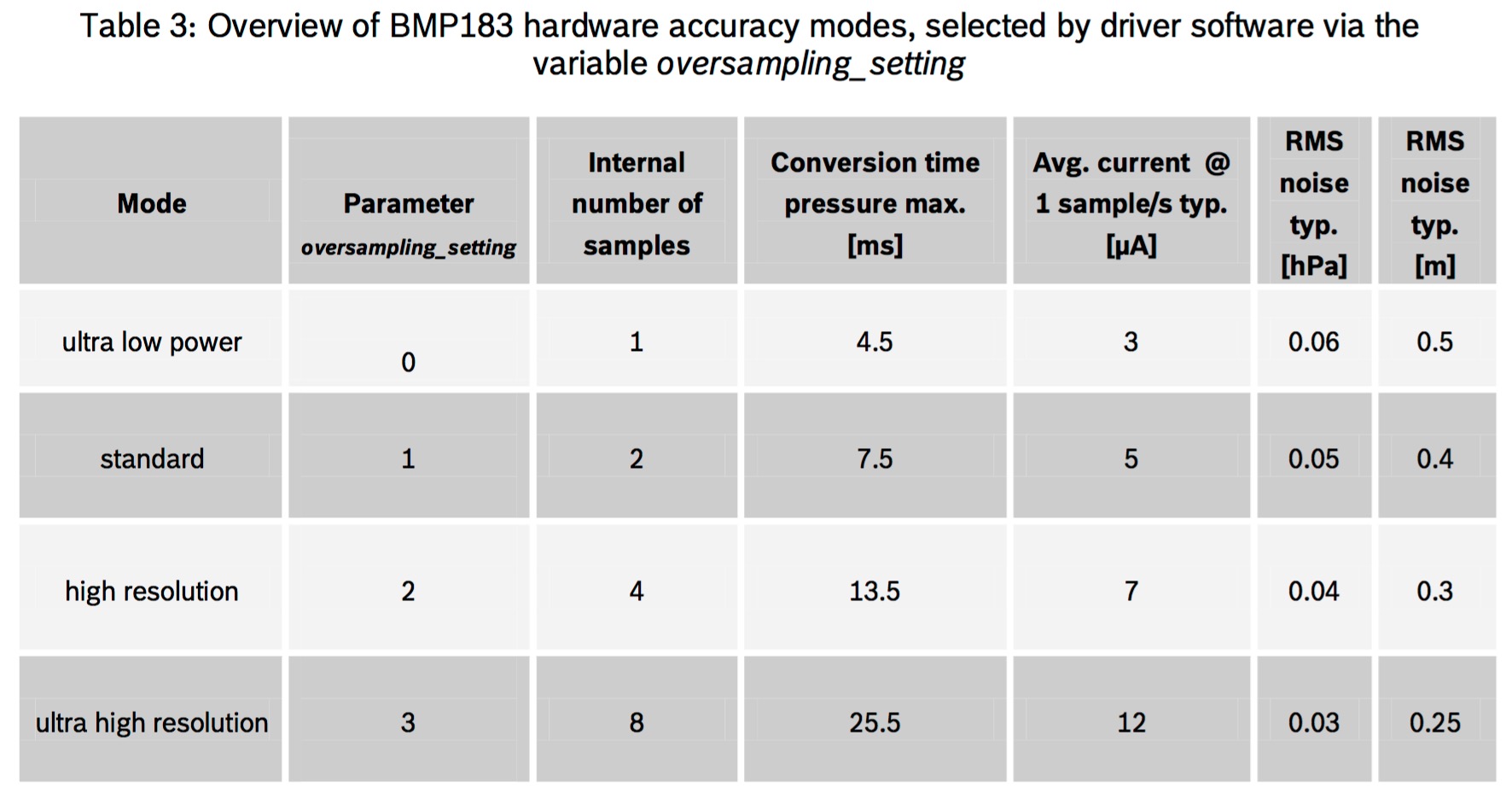
BMP183 Hardware Accuracy Modes
Please right click and open images in new tab for
better viewing.
Lastly, the header file initializes the pressure chip select pin as RPB7 as well as all of the E^2PROM constants
variables and functions that we use in the pressure.c source file. These functions are listed and
explained below:
void pressure_begin(unsigned char); - Sets the oversampling mode and reads out all of
the E^2PROM calibration data.
void spiwrite(unsigned char address, unsigned char data); - Writes the 2-Byte(16 bit)
data to the corresponding address.
unsigned char spiread8(unsigned char address); - Reads the 1-Byte(8-bit) data from the
corresponding address input.
unsigned int spiread16(unsigned char address); - Reads the 2-Byte(16-bit) data from the
corresponding address input.
void delayMs(unsigned long ms); - Creates a millisecond software delay to allow for the
conversion time in oversampling setting modes.
void read_calibration_data(void); - Reads the E^2PROM calibration data and initializes all
of the constants for the specific device used in the temperature and pressure calculations.
UINT16 read_raw_temperature(void); - This function first writes the command to read the
temperature to the control register, 0xF4. We delay for the conversion time and then read the temperature data
from REGISTER_TEMPDATA.
UINT32 read_raw_pressure(void); - This function first writes the command to read the
pressure to the control register, 0xF4. We then delay based on the oversampling mode defined as the conversion
times seen above and then read the pressure data as 3-bytes in order to ensure precision in the high resolution
modes. In the lowest resolution mode, the pressure data is represented by 16-bits while in the highest resolution
modes, the pressure is represented with 19-bits.
float get_temperature(void); - Returns the temperature in degrees Celsius as a float.
INT32 get_pressure(void); - Returns the pressure in Pascals.
float get_altitude(void); // std atmosphere- Returns the altitude form the calculated
pressure. The calculation and relation of altitude and pressure is shown below.
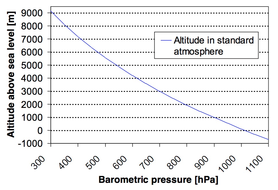
Pressure-Altitude Relation and Barometric Sea Level Pressure Worldwide
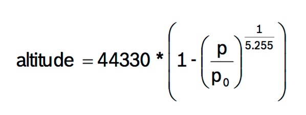
Pressure-Altitude Formula
It is worth noting that in order to get an accurate absolute calculation of the altitude, the barometric sea level pressure is necessary. This value was assumed to be a constant 101325 Pascals. However, in real life this value is not a constant. In fact, it is changing every single day. One way that we could have improved this project would have been to include an input to the system that referred to the local sea level pressure for the specific day. The below graph shows the variation in sea level pressure averages over the entire globe. Clearly, assuming a constant value would produce different absolute results all over the planet. A positive aspect of the pressure and altitude readings were although the absolute pressure was slightly off, the relative pressure and altitude adjustments from point to point were spot on. Changes in pressure, as depicted from the graph above, transitioned nicely into logical changes in altitude. At sea level, a change of roughly 1hPa corresponded to about an 8.43m change. The results section will delve deeper into the successes of the pressure sensor in our test runs.
Gyroscope Sensor
The gyro was a crucial aspect of our project because we needed it to compensate for the effects of gravity and also gave us the rotation around all of the axes. As noted above in the hardware section, the triple axis gyro we used was from adafruit. The chip that we chose supported both I2C and SPI communication so because we had already implemented SPI for the pressure sensor and also to save pin connections, we chose to use the SPI interface.
Following along the standards of SPI discussed above, the gyroscope sensor shared clock and data input and
output lines with the pressure sensor. This is allowed because each chip had a unique CS or chip select line that
limited the devices to be activated mutually exclusively at different times. The gyroscope also came with a lot of
documentation, please refer to specific datasheets for each device in the reference section of this report. Our code
for communication with the gyroscope consists of two files: a header file, gyro.h and a source file,
gyro.c. These and the functions are explained below.
Similar to the pressure sensor header file, in the gyro header file, we first initialized certain mode settings,
important registers, and also pin connections and variables. The mode settings were used to specify the sensitivity
of the device, essentially if we wanted to operate the device on a 250/500/2000 dps or degrees per second range.
We created a typedef enum l3gd20Range_t to associate with the different sensitivity settings and
could be passed as an argument to the initialization function to configure the device. We then defined 15 registers
with their associated values that would be important in the destination addresses for reading and writing SPI functions
. We then defined the chip select pin to RPB5, physical pin 14 as dictated in the hardware section. Finally, we
defined four user functions that are described below:
int begin_gyro(l3gd20Range_t sensitivity); - Enabled all three, X,Y,Z gyro channels, set
the sensitivity of the device to either 250,500, or 2000 dps, and then made sure the gyro was responding correctly.
If the gyro was configured correctly, this function would return a 1, otherwise it would return a 0.
int debug_gyro(void); - Made sure the SPI channel was working and the gyroscope was
acknoledging. Called only in the begin_gyro() function.
void writeGyroSpi(UINT8 address, UINT8 data); - Wrote the data to the gyroscope at
specific address using the standard SPI specification. The address was binary AND'D with 0x7F or 01111111
value so that the most significant bit was a 0, signifying a write operation.
float getGyro(INT16 address); - Retrieved the gyro data for a specific address. In this
case, the address was binary OR'd with the 0xC0 or 11000000 because the most significant 1 represented a read
operation and the second most significant bit incremented the address in multiple readings. The arguments would
be either OUT_X, OUT_Y, or OUT_Z signifying each axes angular velocity. Returned the
corresponding angular velocity in units of degrees per second as a float.
MicroSD Storage
The final device that ran off of an SPI interface was the MicroSD breakout board. This board we got from sparkfun. This particular board ran off of the SPI1 channel and the pin connections are described in the hardware section above. In researching how to interface with the MicroSD and perform read and write operations on data files stored within the FAT32 file structure, we found a project on Syed Tahmid Mahbub's or Tahmid's Blog that read from a microSD. We were specifically interested in the libraries that he used to interface with the SPI protocol. This was Microchip's open source file-system library MDDFS, a part of the Microchip Libraries for Applications (MLA). The files that we used for our project are the same files that Tahmid used for his. From the following folders, we included the following files:
- MDD_includes:
FSDefs.h, FSIO.h, and SD-SPI.h - PIC32:
Compliler.h, FSconfig.h, and HardwareProfile.h - MDD_sources:
FSIO.c and SD-SPI.c
The following section describes the specific sections in the library that we modified to be congruent with our
project. In the HardwareProfile.h header file, starting at line 529, we modified the define variables
to fit with the hardware that we mentioned above. The chip select, chip detect, data in, and data out pins were
configured to our hardware guidelines. The SPI clock frequency we used was 2MHz.
In the MDD_SDSPI_InitIO() function in the SD-SPI.c source file, we set the
MOSI and MISO pins to be used for SDO1 and SDI1. All of the other files, we kept the way they were. The
Microchip library functions that we used are described below. These functions were used throughout the
main.c file and in the microSD protothreads function.
FSInit()- This function initializes the FAT32 file system on the microSD card. It returns FALSE(0) if the initialization fails, and TRUE(1) otherwise. If a microSD card is not present in the holder, the function returns FALSE. This function was called in the main function in a while loop to wait for a card to be inserted.FSFILE = FSfopen(filename, "a+")- This function opens a file to be operated on. The filename is the name of the file that will be saved. The second argument specifies the intended use of the open file, whether it is to be either read("r"), written("w"), or appended("a"). Additional, permissions are allowed to allow both reading and writing or even appending and reading. The function will return NULL if opening the file failed. Otherwise, the function returns a pointer of type FSFILE (defined in the library references) to be used in the FSfwrite() function described next.FSfwrite(buffer, sz, n, FSFILE pointer)- This function actually writes data to the opened file. The data to be written is specified in a pointer of characters that can include data using thesprintf()function in c. The two middle parameters define the number of bytes per input and the total number of bytes to be written. The final parameter is the pointer that was returned from theFSfopen()function.FSfclose(FSFILE pointer)-This function closes the file that was opened through the FSFILE pointer argument.
Python Post-Processing
Due to our technique in integrating the accelerometer data with the gyroscopic data to obtain velocity we opted to do the numerical integration and velocity synthesis in post-processing. Our process is novel and has exciting potential for further work, specifically in improving the accuracy of the velocity estimates.
Methodology
As every physics student learns, acceleration is the first time derivative of velocity. Therefore, in simplest terms, all that is needed to obtain a velocity is to integrate an acceleration function in time. However, there are two rather issues with this approach. Firstly, as Einstein explained to us in his theories of relativity, it is impossible to distinguish an acceleration from a gravitational force in a single reference frame. Secondly, we are not getting literally continuous acceleration data. In the following work, we attempt solutions to both problems as many have before, although perhaps in an innovative fashion.
The first issue demonstrates the necessity of the gyroscope, a tool measuring axial angular displacement. Our solution here hinges on a use-case assumption, namely that the user must be stopped (with a velocity of 0) at the beginning of data logging. This gives us a useful reference point of 0 m/s at the start, which is imperative for our numerical integration to be meaningful. However, as we aren't moving at the start, we can assume that the only measurement our accelerometer will be producing is that of earth's gravity. Therefore, from the first data point of our dataset, we know the initial direction of gravity. From here, we can use the gyroscope to measure the change orientation of our project to keep track of the direction of gravity in the future, allowing us to subtract it out from our calculations, in theory yielding an acceleration that is going purely towards motion and therefore velocity.
The second issue gives way to the most drastic challenges face by the post-processing. As our acceleration data is a set of samples from a continuous acceleration, our integration will not yield completely accurate results. In fact it will yield an ever-accumulating error, which is one of the reasons that integrating acceleration data to get velocity is so difficult and rarely pursued. We make a second assumption here to aid us in facing this challenge, namely that the user will be completely stopped again when data logging is concluded. This now gives us a second reference point from which to work in the analysis of the data, an invaluable tool and part of the novelty of our approach.
Numerical Integration of Accelerometer and Gyroscope Data
Gyroscope data needs first to be integrated in time in order to yield three total axial angular displacement arrays to
be used in gravity compensation. Later the three axial acceleration vectors will received the same treatment, so we
wrote a quick function, included here, that took as arguments the vector to be integrated and the corresponding time
array against which we integrate and returned the integral array.
	def integrate( vect, time ):

    '''This function returns the time integral of vect'''

		   integ = [0]

		   integral = 0

		   for i in range(1,len(vect)):

			      integral += 0.5*(vect[i] + vect[i-1])*(time[i] - time[i-1])   #trapezoidal integral

			      integ.append(integral)

		   return integ
With angular displacement data handy, we can proceed to remove gravity's influence from our acceleration data. To do this, we take the first line of data and, thanks to our first assumption above, take this to be gravity. Propagating forward, we use an R3 three axis rotation matrix to calculate the new gravity axial components at each time step. Improving this step in the process should be one of the primary focuses of further development, as incorrectly compensating for gravity has the potential to produce very misleading results.
With gravity removed, we then integrated each acceleration component in time to produce three velocity arrays, which are then combined using the 3-dimensional Pythagoren theorem at each time step to produce a single net velocity magnitude array. Once correct, as described below, the velocity, temperature, pressure, altitude, and time data are exported to a new CSV file for plotting in your choice of software. For ease we used Excel.
Error Mapping & Optimization of Velocity
With the ability to parse data and produce an initial velocity estimate, our script then moves to correct the ever- present error. To try to estimate the type of error we could expect in our measurements, we held the data logger as nearly perfectly still as possible for approximately a minute four different times, in different orientations, to give use four calibration data sets. We knew that the velocity should be zero over the course of each entire data set, so when we saw the velocity estimate produced we would be able to estimate the pervading error and compensate for it to improve accuracy. Below are the four graphs depicting the uncorrected velocities calculated in each instance.
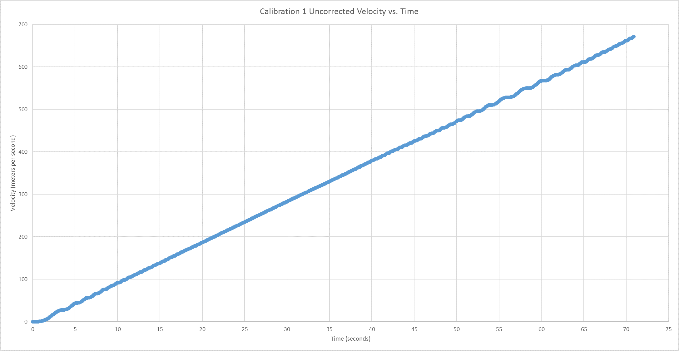
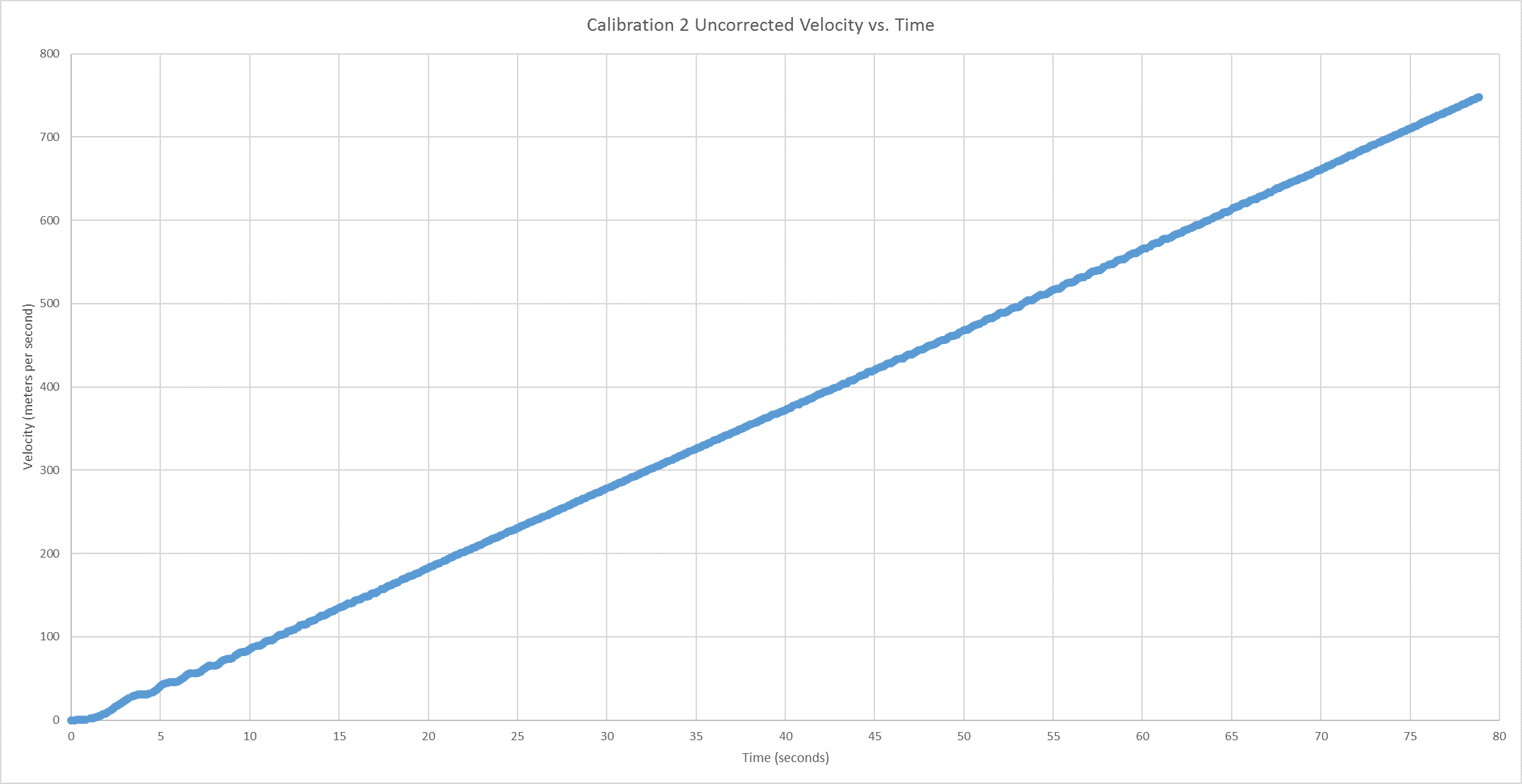
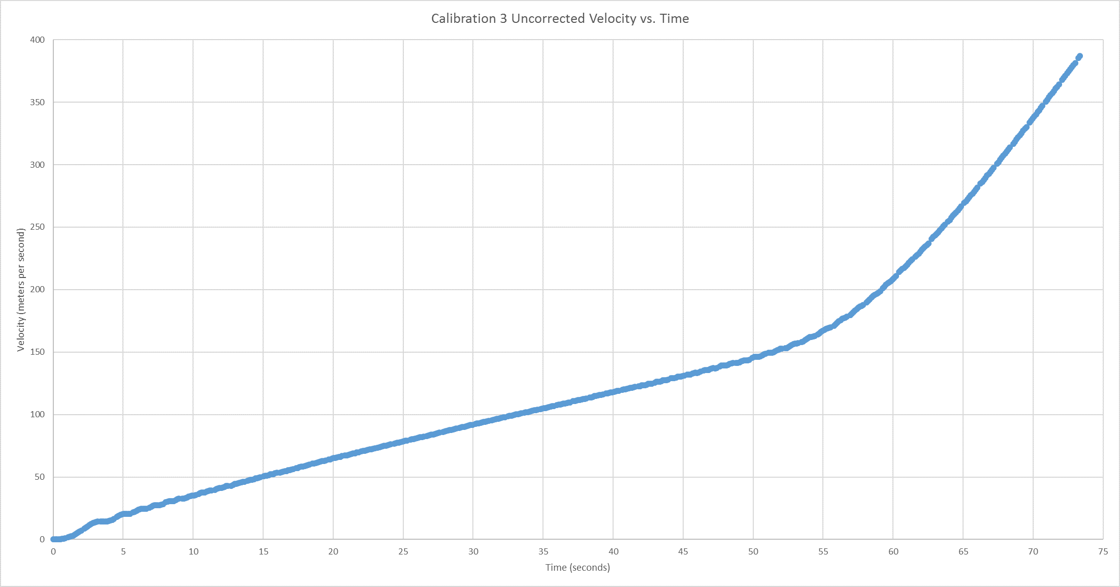
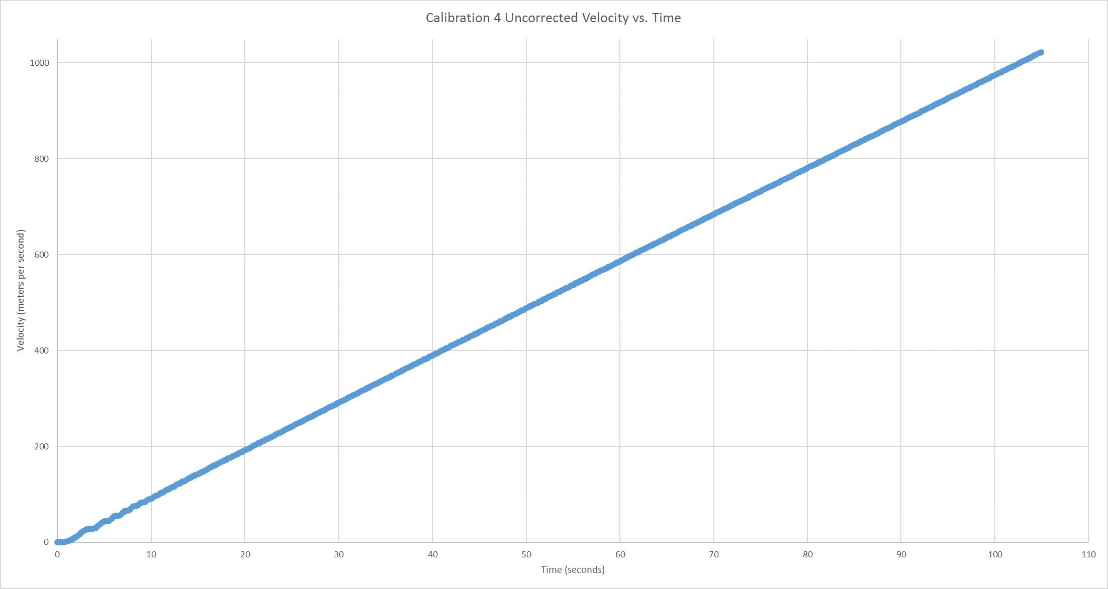
Clockwise from top left: Uncorrected calibration velocities 1, 2, 4, and 3.
Please
right click and open images in new tab for better viewing.
Obviously these velocities get out of hand fast, with calibration set 2 appearing to surpass 1000 meters per second in under two minutes. While we would have liked to explored the almost piecewise nature of the third calibration data set, we assumed it to be an anomalous event and focused on the other three. Specifically we noticed that they were seemingly very linear in their cumulative error. This may make sense if assume a constant acceleration error, which when integrate would yield a linearly increasing error here. Each of their slopes, while similar in order of magnitude, is unique. However, this issue was circumvented by our second usage assumption of no velocity at the stop of data collection. This allows us to apply what we call a 'linear tilt' correction to the velocity. The correction can be pictured as us tilting the velocity plot about a fixed origin until the final point is on the x-axis as we know it ought to be. By applying this fix to calibration data sets 1, 2, and 4 we get the below corrected velocity plots.
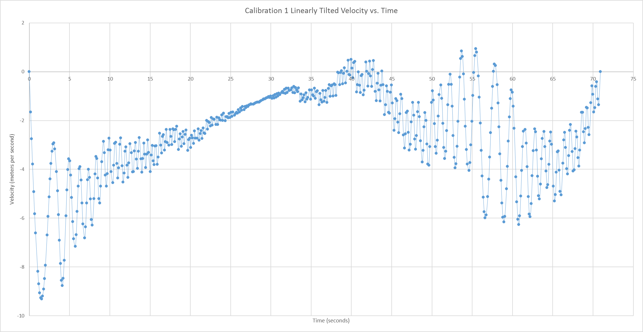
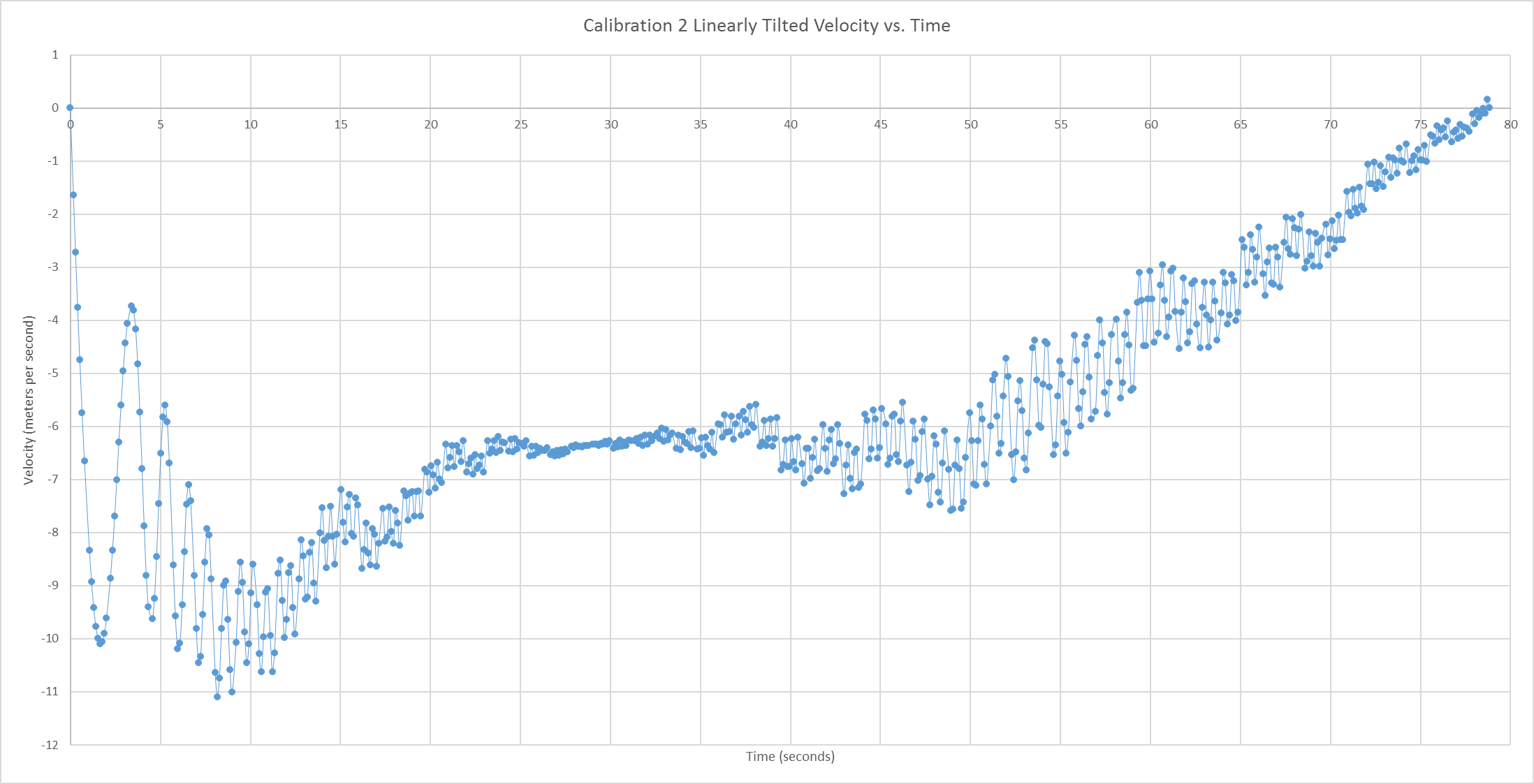
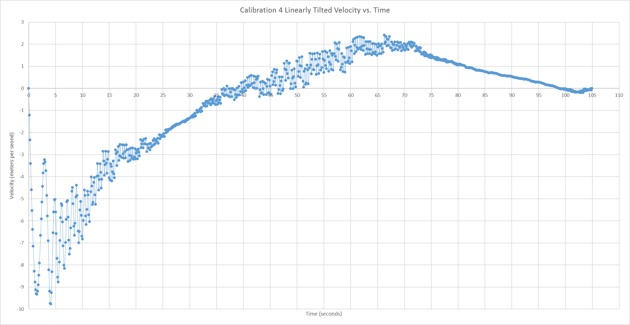
Clockwise from top left: Linearly tilted calibration velocities 1, 2, and 4.
Please
right click and open images in new tab for better viewing.
It should first be noted that this tilt has brought these velocities to a much more reasonable order of magnitude, with only set 2 ever reaching the double digits. Now, while not satisfied with these new plots, we settled with this linear tilt correction fully due to our limited time and resulting inability to further refine this error correcting process. We briefly dabbled with quadratic error correcting under the assumption that there was some linearly increasing cumulative error in the acceleration data resulting in a quadratic change in velocity, but to little avail. Code for this is included but commented out in the downloadable Python script below.There are in fact interesting commonalities between these corrected plots, strongly suggesting a need for further study into our error correction. Of note are the sinusoidal behaviors as well as the 'belts' of tightness all between 20 and 30 seconds.
Results top
Tests
Lab Bench Test
Test done at the lab bench of the finished data logger are detailed in the software section above as the calibration trials. The temperature, pressure, and altitude data from these trial runs is nearly perfectly constant, which we expected, and is of little interest.
Road Test
As of the writing of this report, it has yet to snow in Ithaca. For this reason, and for the aforementioned lack of a proper housing, we opted to test our logger by driving down and uphill while opening and closing the windows to test all of its sensors. We did an uphill and downhill run over the run depicted below at night.
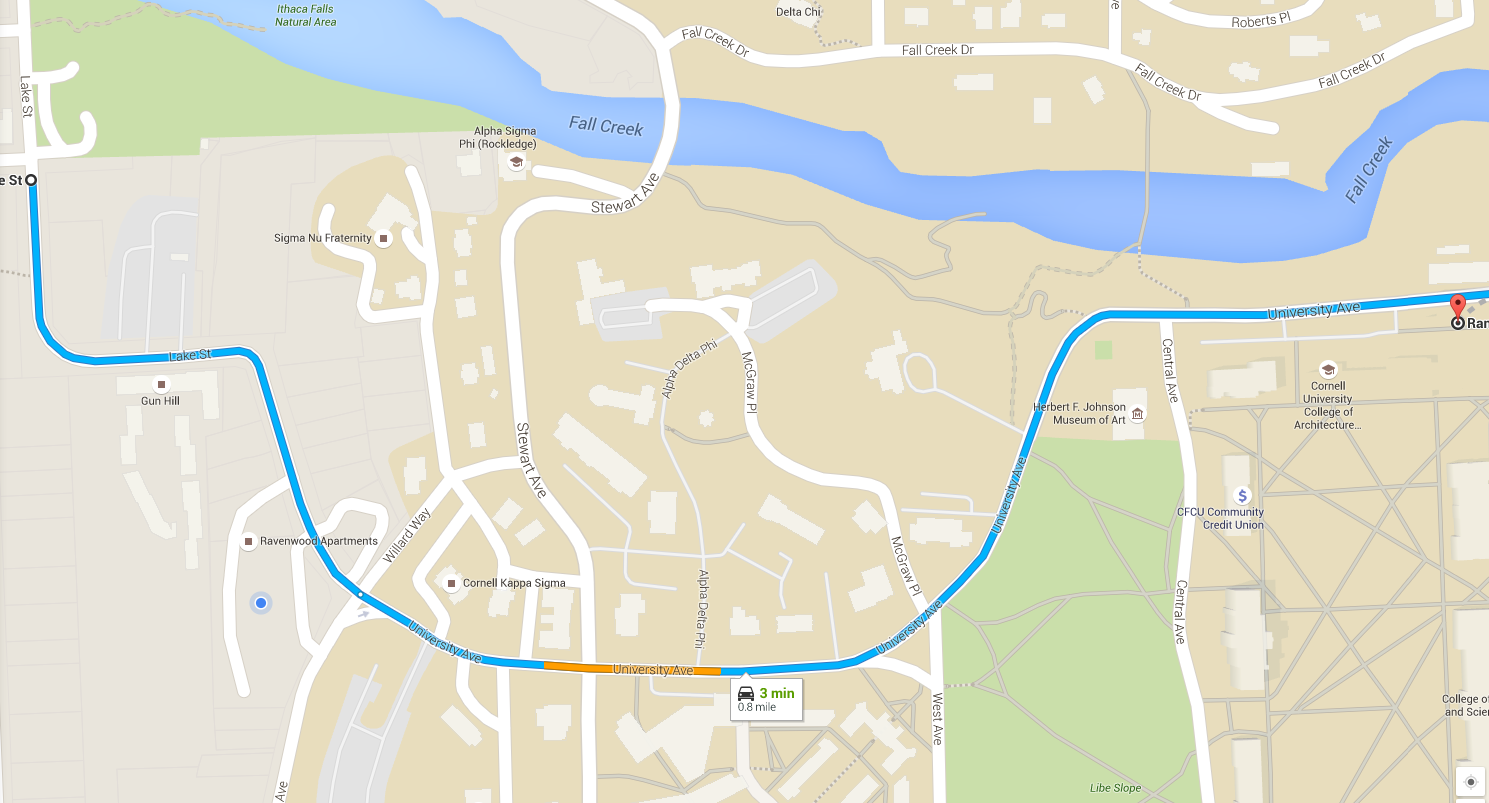
Map of our test run
Please right click and open image in new tab for
better viewing.
This run is almost exclusively downhill with a stop sign at both the intersections with Stewart Ave and Willard Way. Below are included the plotted velocity as well as temperature and altitude graphs of both the downhill and uphill versions of this run.
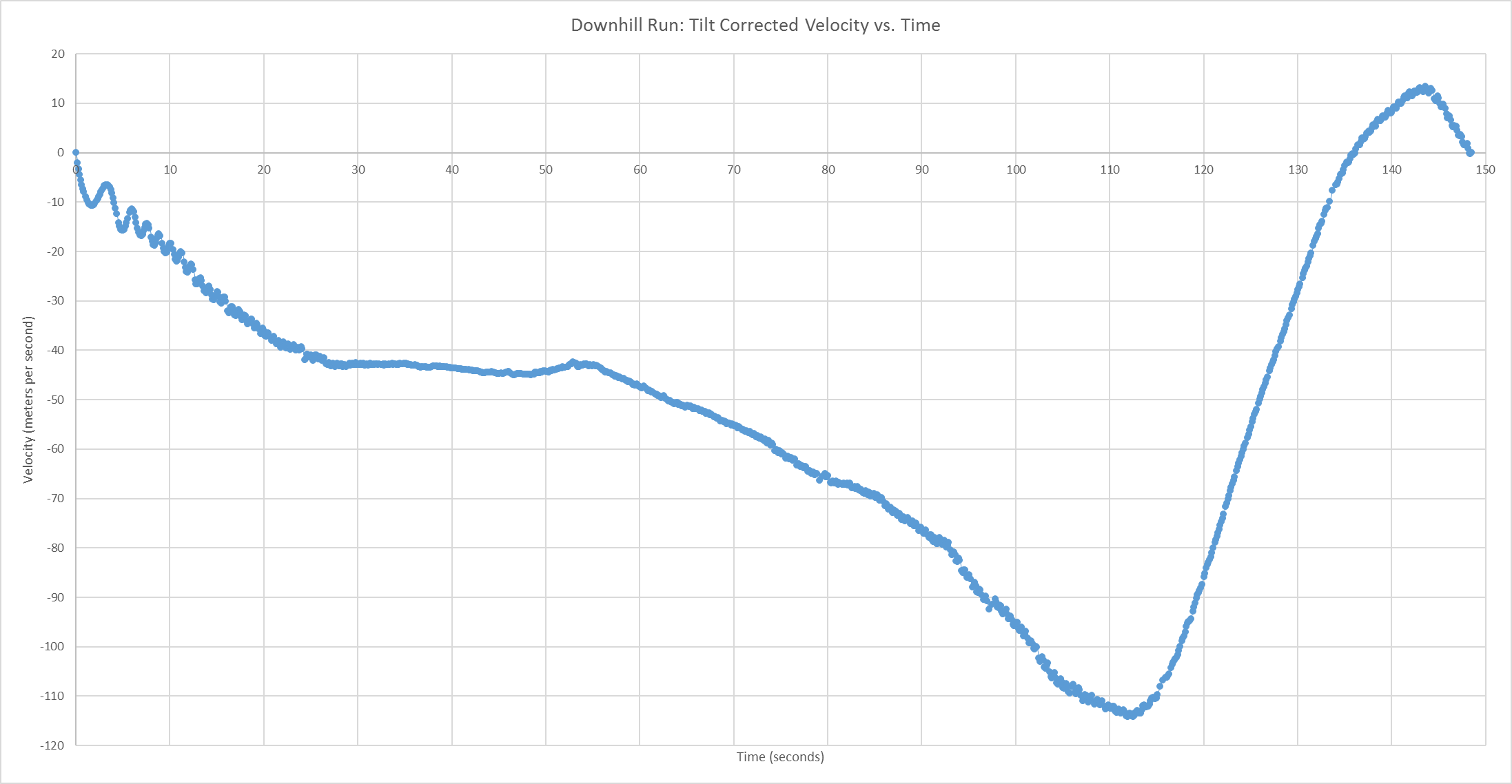
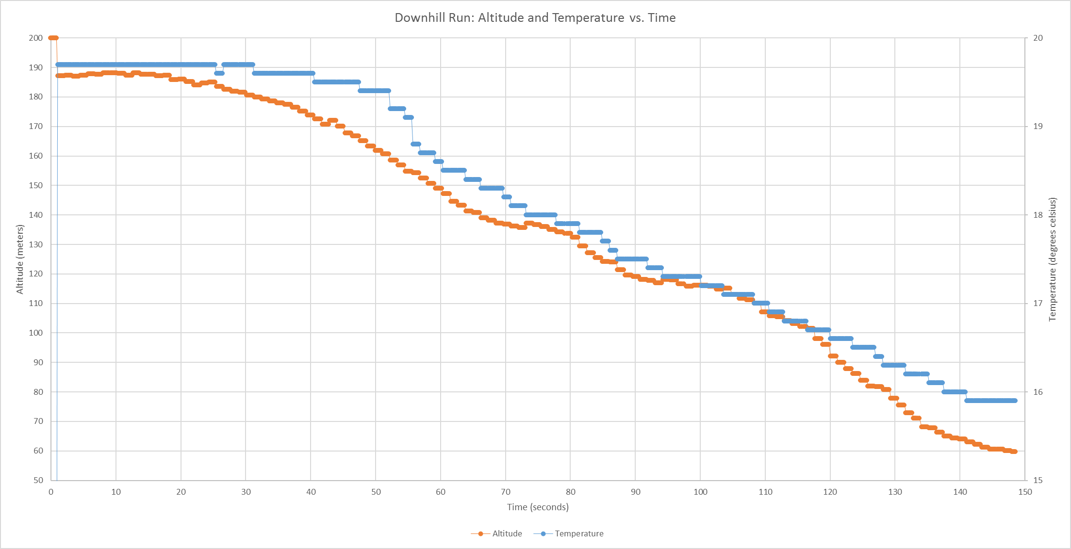
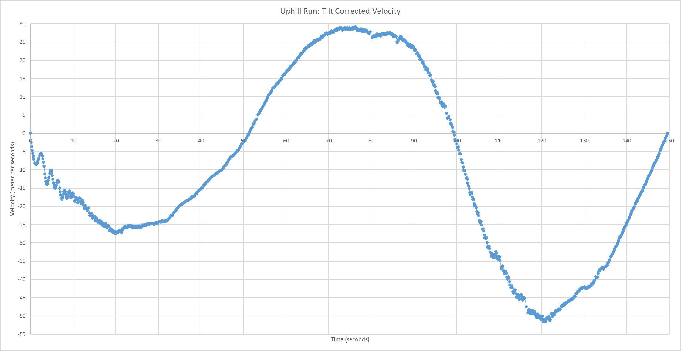
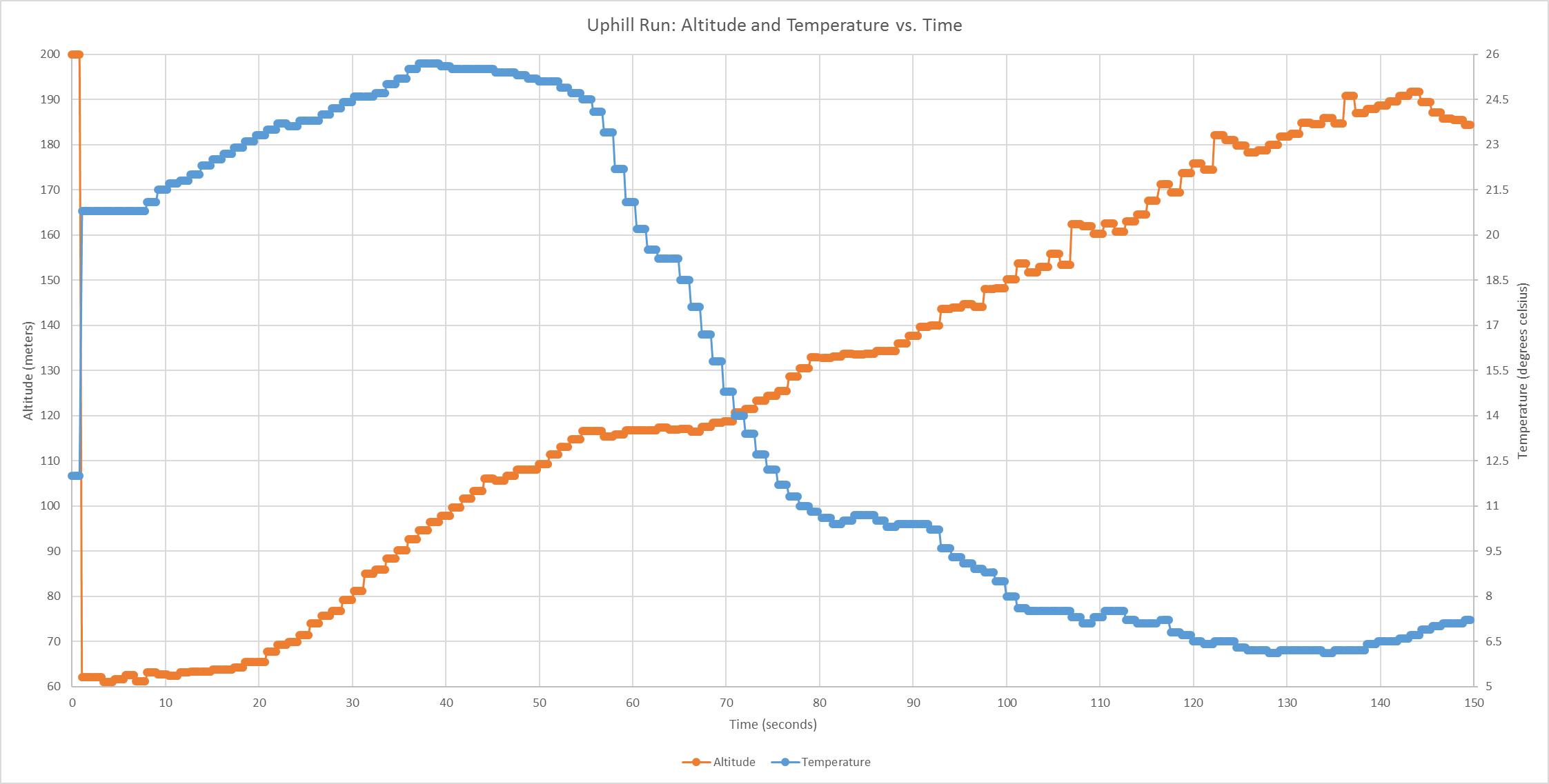
Top: Downhill plots. Bottom: Uphill Plots
Left: Velocity
Plots Right: Altitude and Temperature Plots
Please right click and open image in new tab for
better viewing.
As noted in the software section detailing our post-processing techniques for velocity correction, these plots aren't entirely meaningful. However, they are not devoid of interest, as it should be noted that the uphill plot remains noticeably smaller in magnitude than the downhill plot, meaning our uphill driving speed was slower. This was certainly the case, so while there's still work to be done to improve the velocity measurement's accuracy, it still shows us something.
The altitude and temperature plots are of more interest however, as they very accurately reflect what happened in our tests. As discussed above, the altitude was not absolutely correct due to a lack of real-time knowledge of the sea-level air pressure in Ithaca during our run, but the relative altitude change between start and end of both runs is extremely close to the true altitude change over the run. Also notable is between seconds 40 and 50 in the downhill run when we opened the window of the heated car to the outside cold, resulting in the decline in temperature seen there. On the uphill run we first began reheating the car at full power, which accounts for the clear temperature rise, before again opening the window to witness the temperature drop once again, albeit this time more steeply. The window was rolled up just at the end of this uphill run, once again accounting for the slight upward trend over the last twenty seconds.
Safety
Safety was a major concern for us with our initial project proposal. Because we wanted to have a heads- up-display, we needed a small enough screen set in the peripheral vision of the user so that it would not be distracting or get in the way during live activities. After a lot of thought and consideration, we decided that this would not be a good idea. We were not able to find a screen smaller than an inch which would still take up a lot of space when put in front of someone's eye and inside a ski goggle or helmet. Therefore, we decided to ditch the idea of a screen that provided real-time updates altogether. After this adjustment to our project, there are no other safety concerns other than possible electrical contact with skin.
Usability
We tried to design this project with usability in mind. Obviously, there are improvements that could be made in this regard, but overall the device was fairly easy to use. Once power was supplied to the microcontroller, one just needed to insert the microSD card and it would begin logging data. It would have been nice if we put the hardware and sensors on a solder board, enclosed the system with an external battery power supply and switch to turn the system on and off so that it could be shielded from the elements. Another feature worth implementing would be a mechanism by which you could stop one data logging to later start another, saving multiple runs in uniquely named CSV's.
Conclusions top
General Results
Our design worked nearly as anticipated. As discussed, the velocity synthesis has work yet to be done on it, but aside from that our data logger runs perfectly. Temperature and pressure data are taken perfectly, yielding a very accurate altitude measurement as well. Our SPI communication with the SD Card reader, used to create our data logs in the CSV file format, was completely successful as well. The biggest issues we ran into over the course of this project involved getting the nuances of each SPI protocol for each different device using it to work and the designing of a velocity synthesis algorithm. We spent a great deal of time reading data sheets to find the names of specific registers for various sensors as well as troubleshooting SPI signals using an oscilloscope. Other troubles along the way included breadboards which had power rails discontinuous in the middle unbeknownst to us as well as broken ground wires.
Intellectual Property
With further development, we believe that there is a possibility for our synthesis of velocity given both acceleration and gyroscope data to be patented. Based on our research online, it is a rather novel approach to the integration of the two data given our usage assumptions. We would be interested to hear from anyone should they pursue this further themselves, and may update this project in the future with our own work.
Legal Considerations
All software tools we used, such as the MPLab IDE, Python, and various software libraries, are freely available to the public. As such we do not believe that any of our work violates any intellectual property rights or laws. We also believe our final logger to be dissimilar enough from anything existing on the market today so as not to be problematic.
Ethical Considerations
Having switched from a heads up display to a data logging tool, as well as the usage assumption (which would be included as an instruction in any commercial release) of being still at start and stop of data logging, we feel comfortable that our project cannot make skiing any more dangerous than it already is. Without endangering anybody, we don't feel our project to be in any way unethical.
Appendices top
A. Program Listing
The below first link contains the project code that was run on the microcontroller. The second link is to the Python script used to parse the CSV files from the MicroSD Card.
PIC project download herePython data parser download here
B. Schematics
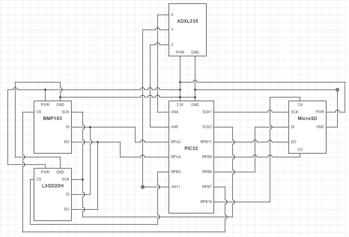
Project Schematic: This schematic more thoroughly details the pins
we used for each of our connections.
Please right click and open image in new tab for
better viewing.
C. Parts List
| Part | Vendor | Cost/Unit | Quantity | Total Cost |
|---|---|---|---|---|
| PIC32MX250F128B Microcontroller | Lab | $5 | 1 | $5 |
| MicroStick II | Lab | $10 | 1 | $10 |
| White Board | Lab | $6 | 1 | $6 |
| BMP183 Pressure Sensor | Adafruit | $9.95 | 1 | $9.95 |
| ADXL335 Accelerometer | Adafruit | $9.95 | 1 | $9.95 |
| L3GD20H Gyro | Adafruit | $14.95 | 1 | $14.95 |
| MicroSD Transflash Breakout | Sparkfun | $9.95 | 1 | $9.95 |
| 8GB SD Card | Best Buy | $4 | 1 | $4 |
| TOTAL: | $69.80 |
D. Division of Labor
Almost all of the project, from design conception, to writing the code, and implementing the hardware design, was all done together. However, there was more focus for Matt on writing the PIC code and implementing the SPI communication protocols. Aidan focused his work on the python post-processing script. Both parties spend a great deal of time debugging as the project progressed, both separately and together.
References top
This section provides links to external reference documents, code, and websites used throughout the project.
References
Acknowledgements top
We would like to thank Bruce Land for a great class and for all the help and guidance offered throughout this project. We would also like to thank our lab TAs, specifically Shiva, for helping us debug our work and keeping the lab open for so many hours.
