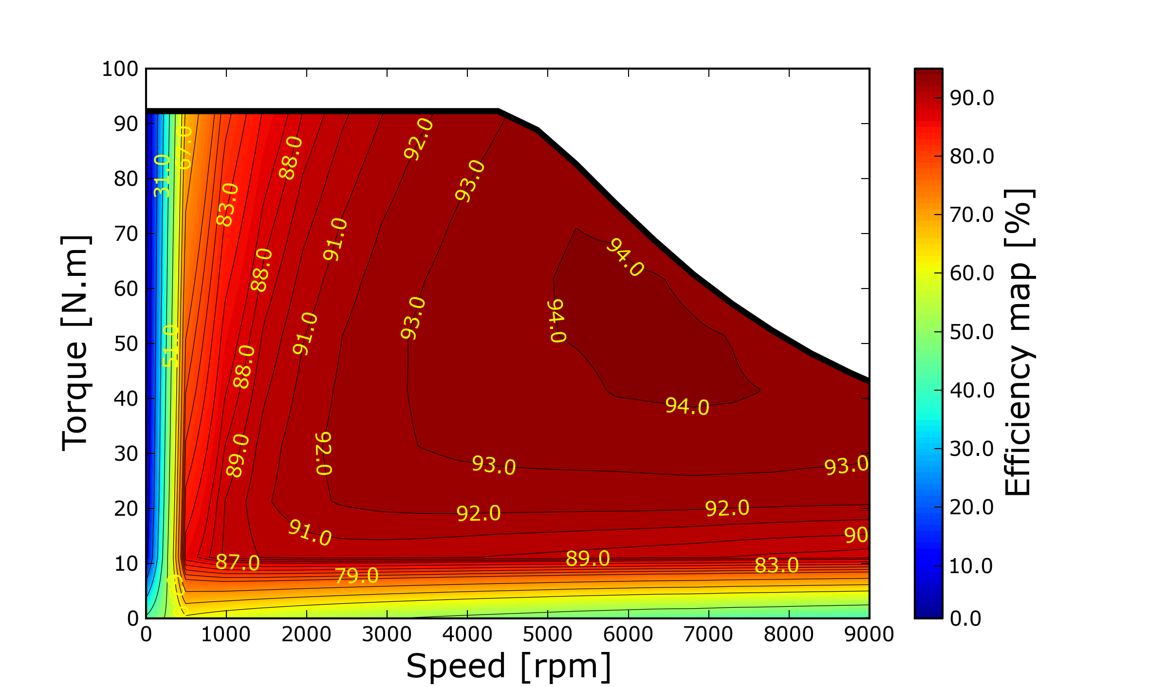
For our final project we built a dynamometer that measures various performance characteristics of small electric motors, such as torque, rpm and efficiency. The final goal was to be able to produce a motor efficiency map like this one, but for this class project the goal was just to get everything designed and functioning:
The main motivation for this project was that two of us are on Cornell's Resistance Racing project team. Resistance Racing participates in the Shell Eco-Marathon, a competition where teams compete to build the most energy efficient vehicle. Therefore, a dynamometer is an important tool in selecting the right motors and tuning our custom motor controller. It would be able to inform us the most energy efficient way of accelerating our vehicle, such as when to turn on the motor and how much current to send at what rpm. The competition requires an average speed of at least 15mph, so the right strategy can really benefit us in using the least amount of power to maintain that speed. Most experienced teams use anywhere from 800W to 1.5kW motors, so we sized our components accordingly.
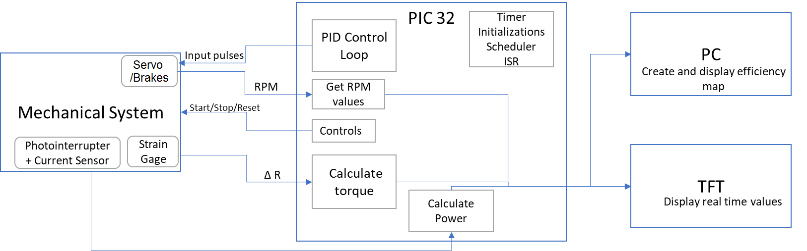
There were many systems in this project, each focusing on one sensor to measure a value required in power calculations. To calculate efficiency we must know the input electrical power, measured by the voltage and current of the power supply, and output mechanical power, given by the torque and angular velocity of our motor. We measured the current using a Hall Effect sensor, torque using strain gauges, and RPM using an IR sensor described in further detail below. The sensors were housed in a mechanical setup with one spinning shaft spun by the motor and one stationary shaft where torque measurements can be taken.
There weren't many commercially available small scale motor dynamometers on the market, only one that we could find sold by a specialized testing equipment company, and there were no DIY/maker project of this variety that we could find for collecting data. Moreover, most dynamometers used complex and expensive water/eddie current brake systems instead of a pure friction based one like this. So this would be one of the first student/maker projects in making a friction-brake based electric motor dynamometer. To test the system, we used a brushed 540 DC motor rated at around 300W and 0.1-0.2 N-m of max torque.
Our project idea came from our participation in the Resistance Racing team. Larger dynamometers were commercially available, however, the team wanted to construct its own version that could be used in testing motors with different specifications.
The structure of our code was relatively simple in that most of the sensors run independently of one another, although they were connected by the mechanical setup. This allowed us to use a bottom-up method for programming our system; we wrote seperate scripts to test each sensor and, after those were debugged, integrated them together into a single program. The most tedious background research we had to do for this project was figuring out how to get data from the strain gauges. We researched the benefits of the different configurations of the wheatstone bridge (whose math is explained below) and decided on a half bridge. Other tradeoffs we cosidered were mechanical complexity for each choice of sensor. This problem was especially important in our determination of what type of IR sensor to use.
The standards relevant to this project include the Universal Serial Bus standard and protocol to serially communicate and transfer measurements to the PC. The ASTM E251 standard for strain gages will be used as a reference for building the strain gauge based torque sensor.
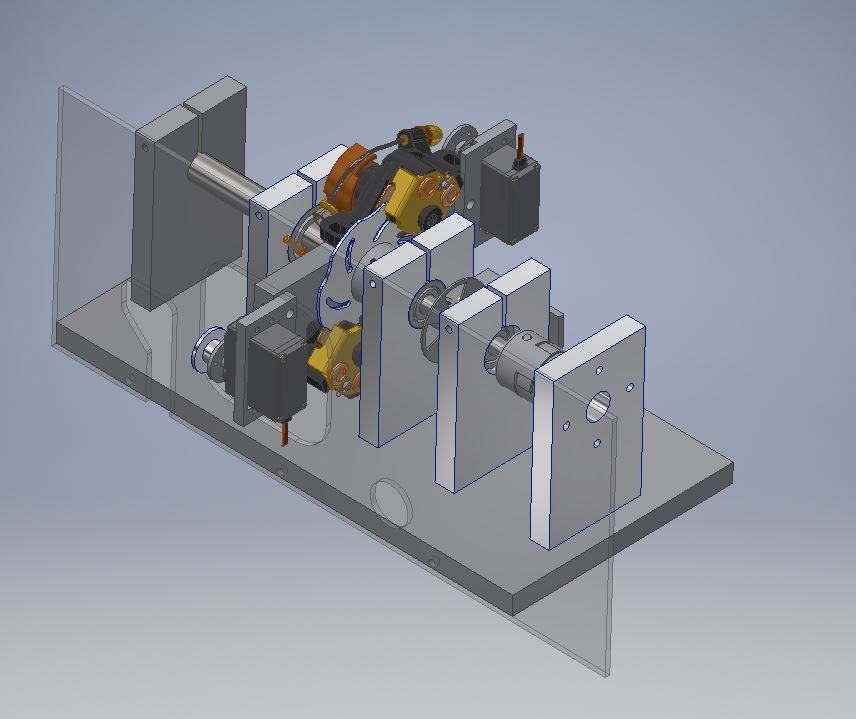
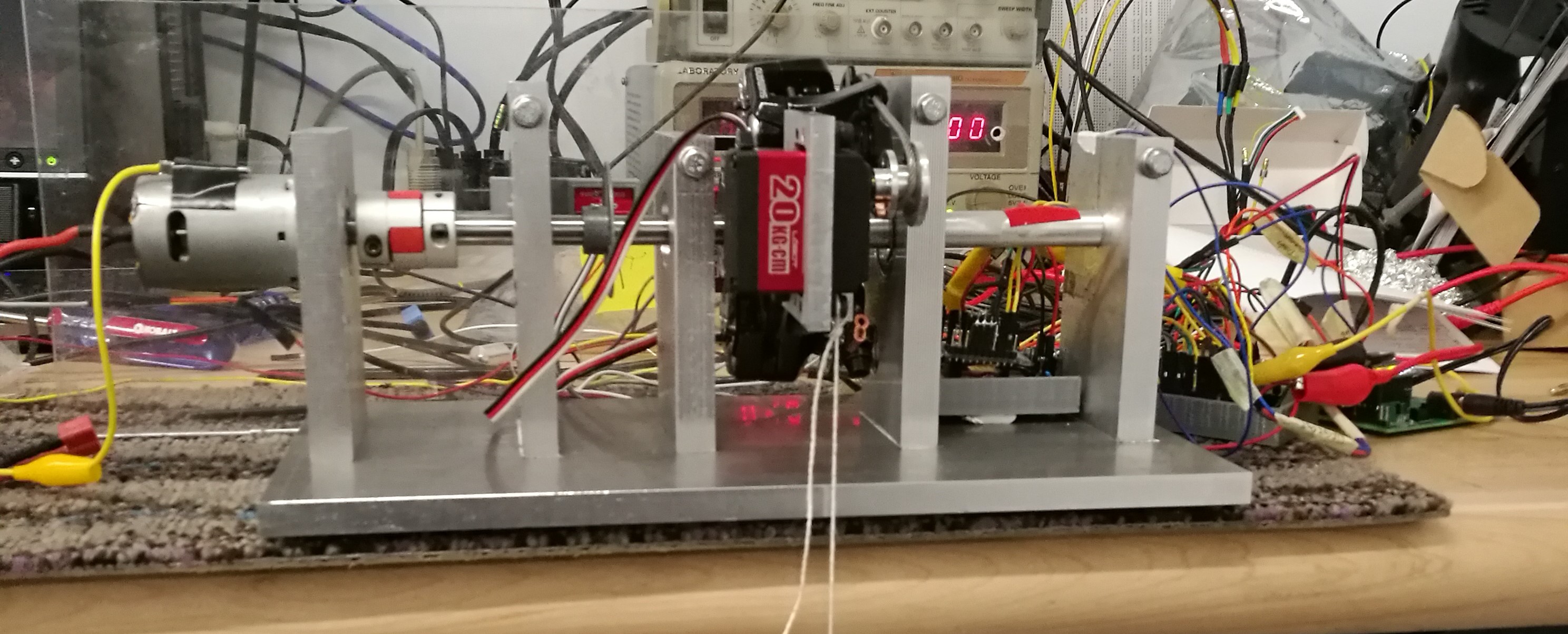
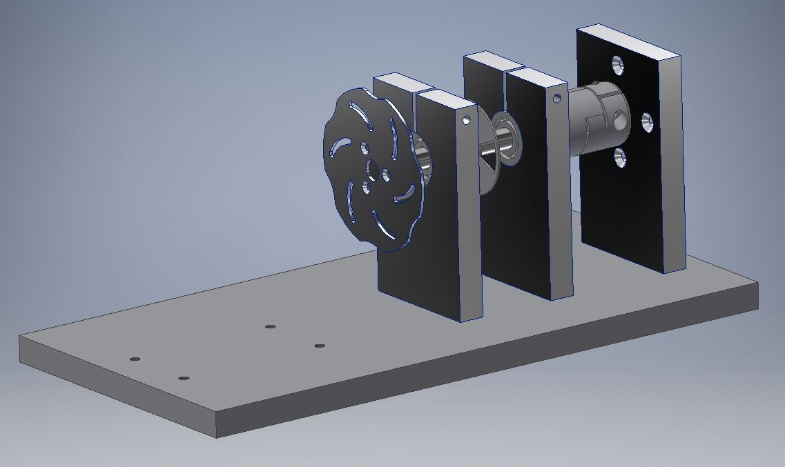
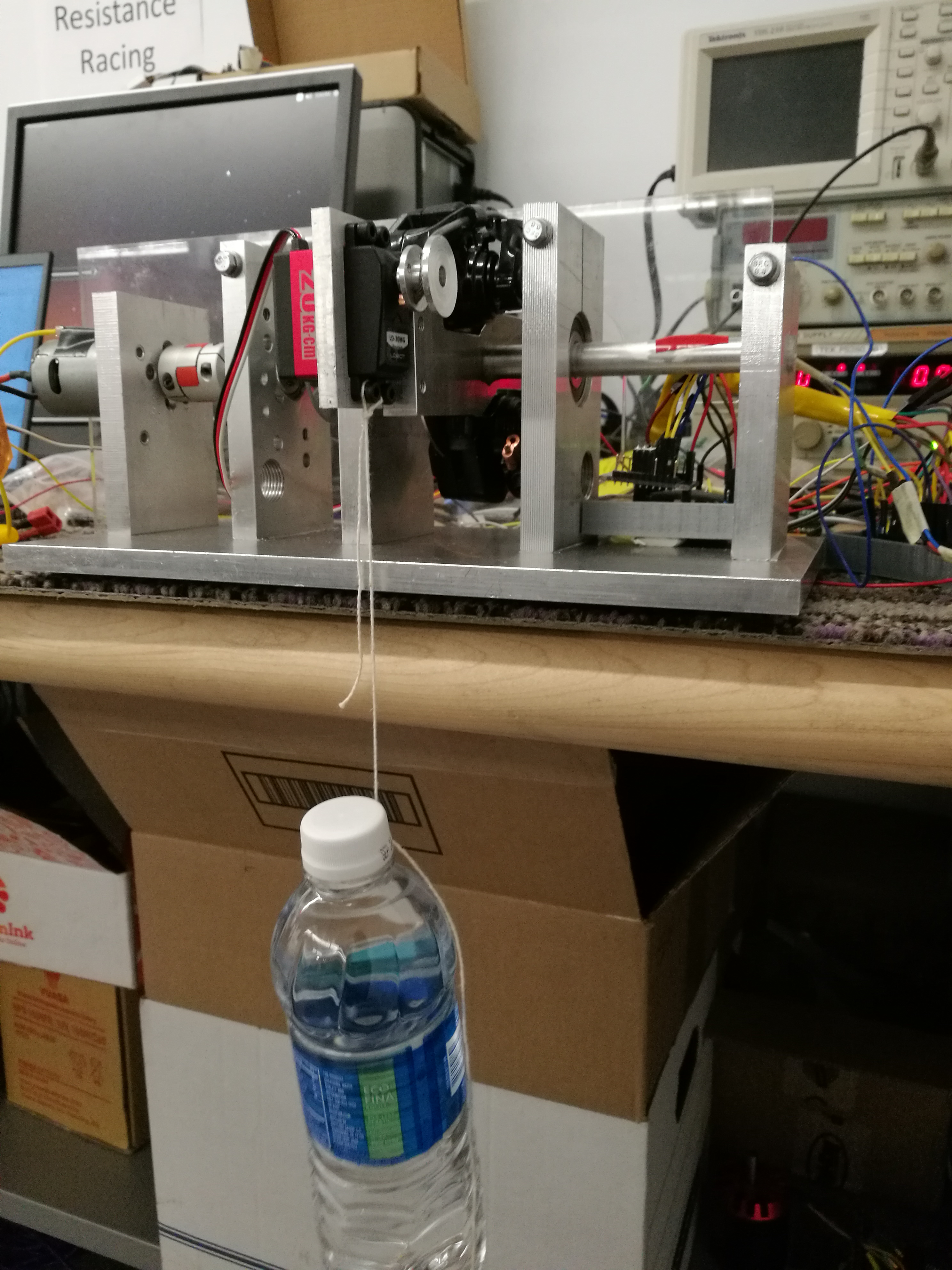
The hardware for this project is a mechanical setup consisting of a metal base plate and five supports. Images of our final setup is shown below, together with CAD renderings:
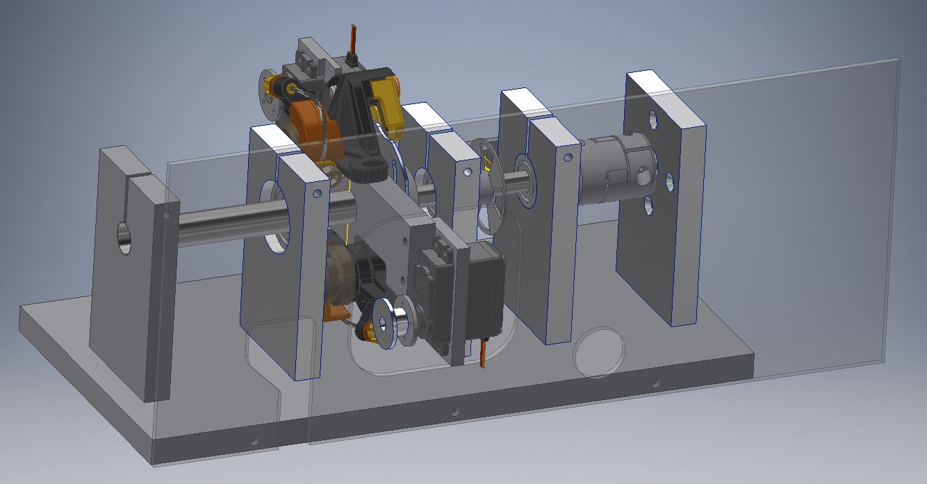
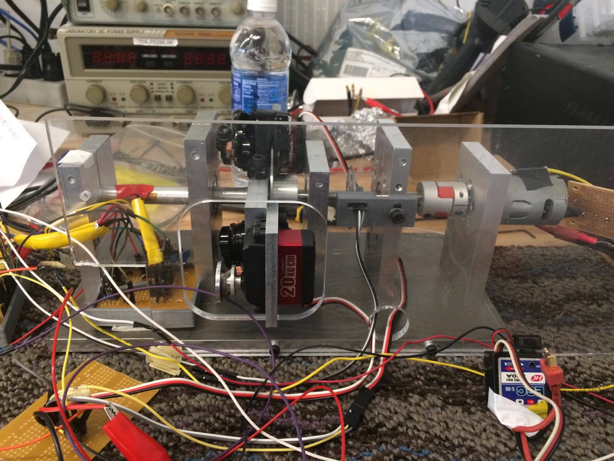
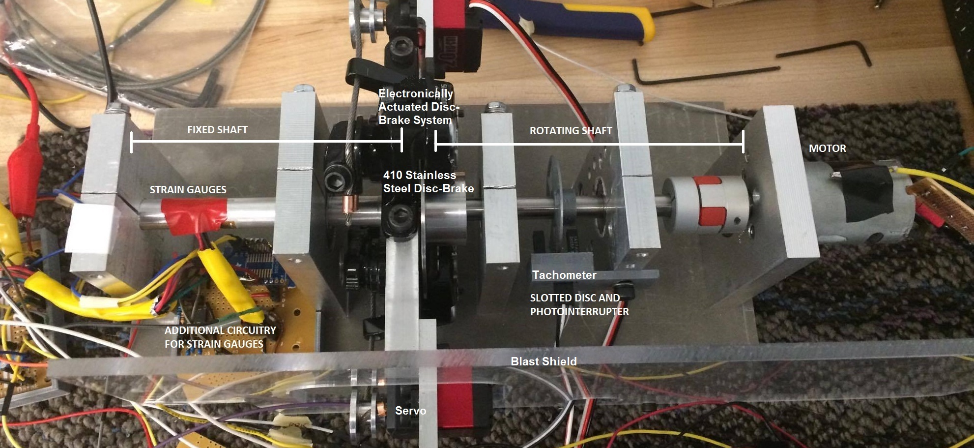
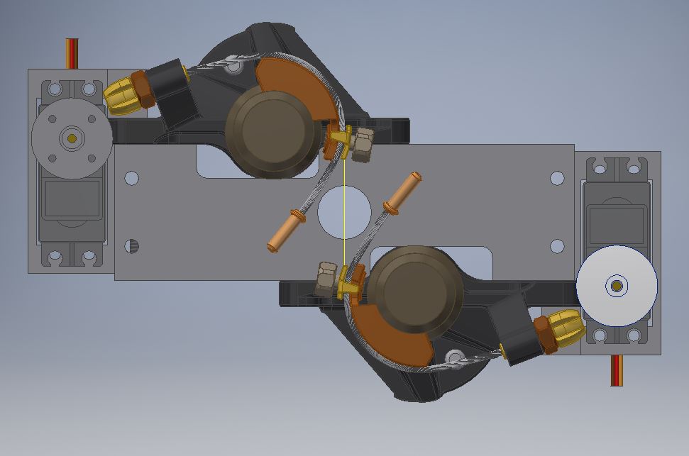
The setup consists of two coaxial shafts, one fixed and one free to rotate, secured radially by large roller bearings. The supports (except for the motor mount) are slotted to allow for clamping on the shaft and bearings for retainment. The solid shaft is attached to the motor via a lovejoy-style shaft coupler and rotates freely, but is axially constrained by the motor. For RPM data collection, a 3D printed slotted disc is fitted over the rotating shaft and a photointerrupter is mounted on to the supports such that it is "interrupted" by the slotted disc. As the shaft spins, the obstructions and slotted areas of the disc change the voltage read by the receiving end of the photointerrupter, allowing us to track angular speed. The other end of the free shaft, in the center of the mechanical setup, is a 410-stainless disc-brake that rotates with the shaft. It interfaces with the electronically actuated brake system, on which two servos control a set of bicycle brakes (by pulling on steel braided wires) to deliver load on the disc-brake. The actuating portion of the brake system is attached rigidly (with epoxy) to a thin aluminum tube which is fixed via clamping on the other end. The strain gauges are then mounted on the thin aluminum tube, where they are able to sense any material strain due to torque. Because the measurement shaft is fixed radially, any bending and off-axis loads will be negated by the bearing support and will not influence the section of aluminum tube onto which the gages are attached. Here is a clear rendering of the fixed servo-brake system:
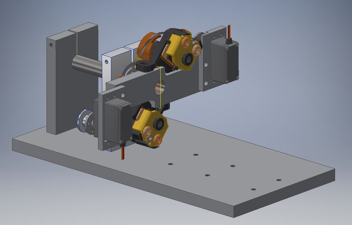
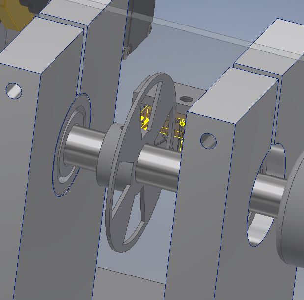
And the rotating portion that is being braked (Note: motor not in rendering):
The disc itself is attached to an aluminum adapter with flathead screws for clearance, which is then fixed on the rotating shaft with a set-screw. Care was taken in the design stage to make sure all interfaces can be assembled smoothly and any alignment errors can be adjusted manually. For example, the through holes in the bottom plate were made extra-large to allow for compensation of the shaft concentricity in multiple axis. Moreover, extra room for the purchased bicycle brakes allowed us to fine tune both the brake clearance and engagement so both calipers exerted approximately the same load.
Engineering drawing were made from the CAD model and almost everything was custom machined by us and Resistance Racing team members in Cornell's Emerson Machine Shop. The bottom plate was made out of solid 6061 T6 aluminum, and so were the 5 motor/bearing stands. The rotating shaft was a piece of tight tolerance high-speed-steel, and the brake-shaft adapter was made from 6061 aluminum. The main body of the brake system was milled out of a chunk of 7075 T651 aluminum stock, and the servo mounts were made out of 6061 aluminum. The brake disc itself was made from 410 stainless stock, which we CNCed in order to obtain +- 0.001" flatness with the circular profile (measured on a lathe with dial indicators). The fixed shaft is a piece of turned and sanded aluminum 3003 thin-walled tube, which was chosen specifically for its strain under torsion, detailed in the next section.
We chose to manufacture almost everything out of metal since we want the best rigidity under dynamic loading conidtions. For the brake, 410 stainless was chosen because it is wear-resistance and a common material for bicycle disc-brakes. For the rotating shaft, we chose a very hard and tough steel since we did not want it to wear and cause vibrations. Some members of the project team also ran some thermal calculations on the disc-brake, and it was capable of dissipating 2000W+ for 5-10 seconds without getting excessively hot (<100 Celsius). Lastly, we ran some statics calculations on the fixed shaft and disc brake epoxy joint, and with our choice of gorilla epoxy, there is a safety factor of over 7 with 5 N-m of torque (our upper range of motor torque measurement).
In terms of the electronic hardware, the intrumentation circuitry for the strain gauges was attached close to the mechanical setup to eliminate noise that may arise from long wires. Any critical signal wires carrying micro-volt signals were shielded and grounded with an aluminum foil jacket. The circuitry used includes a wheatstone bridge and instrumentation amplifier as described in the sections below. The RPM/angular speed is captured by a photointerrupter, the current is being read through a hall-effect current sensor, and the supply voltage is measured from a voltage divider directly into the PIC32's ADC. Custom 3D-printed enclousures for each circuit board was design and mounted as well. The instrumentation amplifier used is the INA121 from Texas Instruments, the digital potentiometer used is the AD5231 from Analog Devices, the strain gage used is the EA-XX-125TK-350 from Vishay, the current sensor used is the ACS758 from Allegre MicroSystems,and the photointerrupter is the GP1A57HRJ00F from Sharp.
Although the system would function on 2 power supplies, we opted to go with 4 due to adjustability. The high-current supply was used to drive the motor, capable of drawing over 20 amps. The low powered supply was used to drive the servos, which operate best at 6V. One triple output power supply was used to drive the instrumentation amplifier and the digital potentiometer at +- 3.3V, while another acted as the excitation supply for the strain gages. The reason why we used 2 triple-output supplies was because we decided to filter the excitation source, which dropped the supply voltage going into the wheatstone brdige and thus needed to be turned up to 8-10V for the same results.The second triple supply was also used to power the cooling fan for the motor.All the grounds are connected together for common ground with the MCU ground, especially important for the instrumentation amplifier and the ADC.Care was taken so that the higher voltages were isolated and would not fry the MCU.
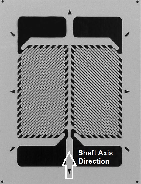
In order to measure torque and strain on the shaft we used two strain gauges (packaged into one pad), which measure small values of strain on an object. As torque is applied to the shaft, the foil/wire that makes up the strain gauge undergoes tension or compression which results in a change in electrical resistance.
To measure change in resistance, we use the gauge factor, a property that determines sensitivity of the gauge. The gauge factor, GF is equal to the change in resistance divided by the resistance at no load divided by the strain. The equation is:
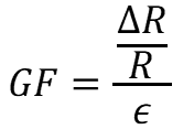 . The standard gauge factor used is 2, and the change in resistance can be as small as microhms.
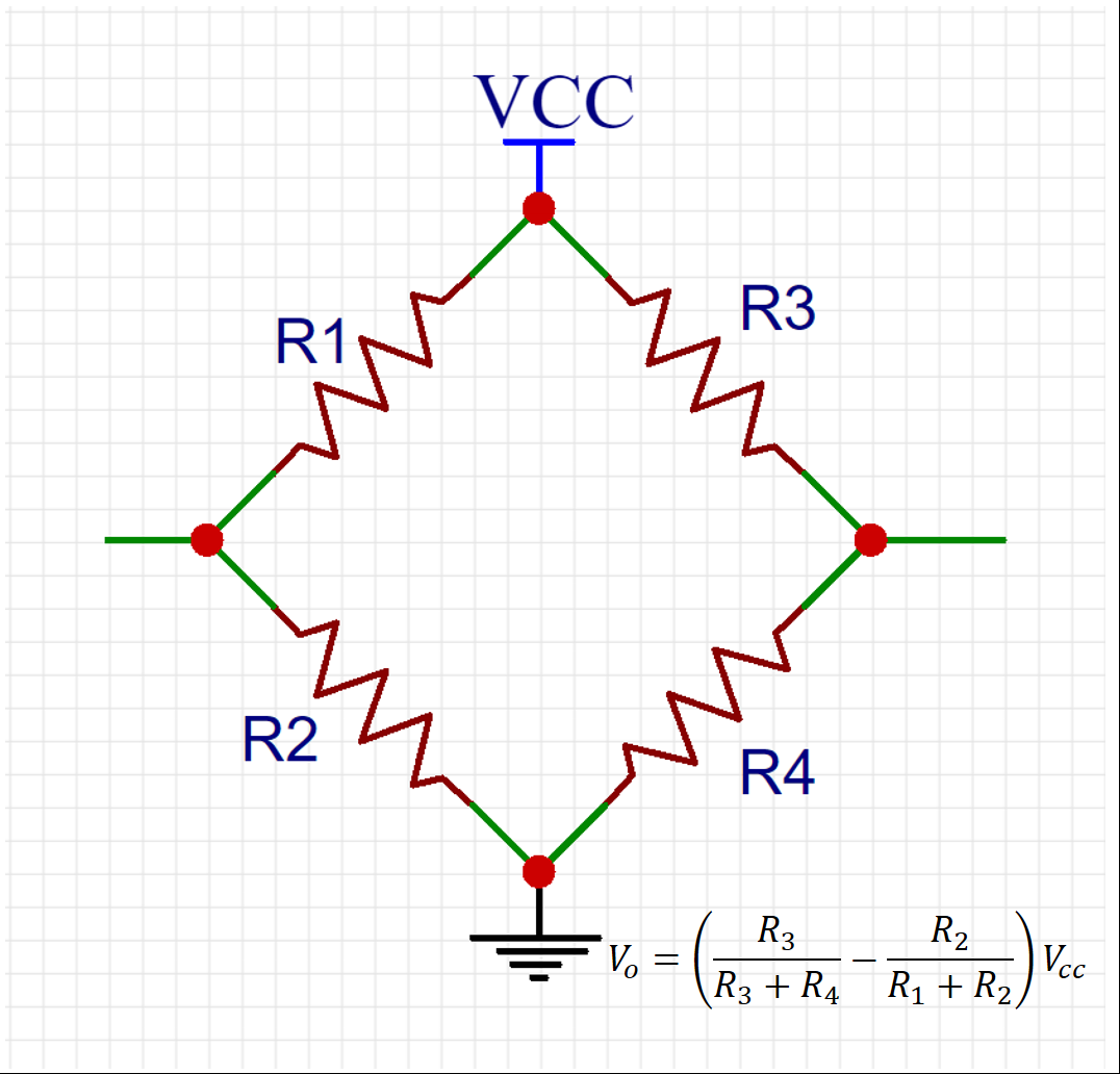
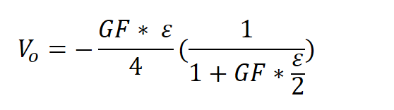
To measure such small changes, a wheatstone bridge circuit is traditionally used. A wheatstone bridge circuit balances two legs of a bridge circuit in which one or more resistances can be variable.
A simple example is the quarter bridge circuit in which there are three passive resistors and active resistor:
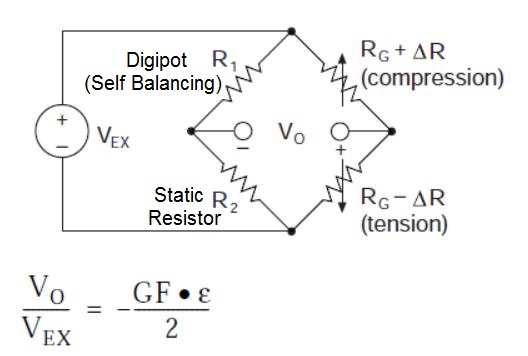
Before we tested with strain gauges, we built a quarter bridge with a 10K potentiometer as our active component. We achieved a gain of approximately 100 with this test circuit, so we then mounted two strain gauges on the shaft, and transferred our circuit to a breadboard. However, we found that the potentiometer was difficult to tune and keep stable.
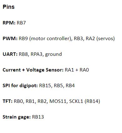
To achieve finer resolution, we used a digital potentiometer which has 10-bit resolution for the self-balancing quarter of the static half of the bridge. We interfaced with the potentiometer using SPI, and used the chip select (RB4), Clock (RB15) and Serial Data Output (RB5) on the PIC32. By sending 32 bit control words with MSB as 0xE or 0x6 (as seen from AD5231 data sheet), we can command it to either increase or decrease the resistance by 1/1024 levels. Combined with a simple conditional statement in a loop, the circuit becomes self balancing. By putting this 10k digipot (measured 8.6k) in series with 15 kOhm resistors (one quarter of the bridge) and balancing that against a 20 kOhm resistor (the other quarter of the bridge), we were able to achieve a theoretical balance accuracy of 0.05%. In practice it was closer to 4-5% accuracy, possibly due to noisey power supplies or amplifier drift.
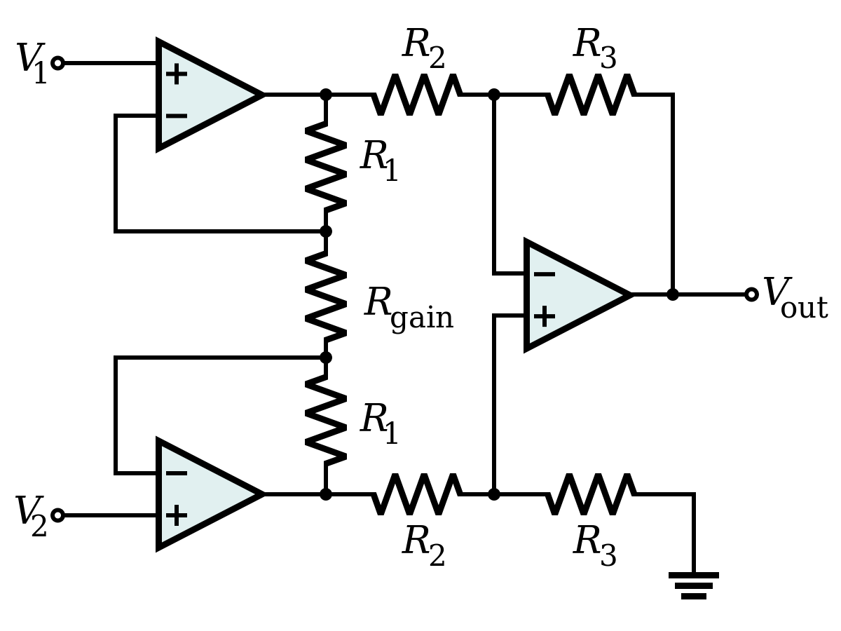
Our final circuit design with adjusted resistor values was the following:
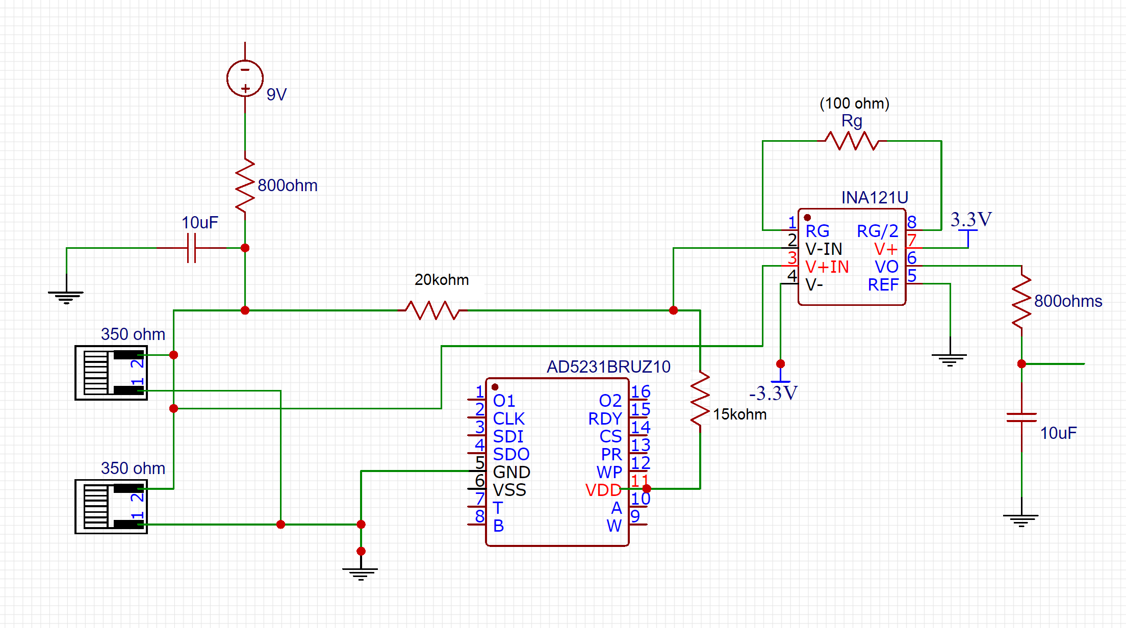
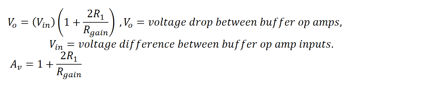
The labeled instrumentation circuit minus the filters can be seen below:

The output of the instrumentation amplifier plus filter is wired to the third ADC channel on the PIC. In the currSensor thread, the raw adc value is read approximately 120 seconds after the program has started. The raw_p value is used to determine and filter the strain on the shaft. The equation for this IIR filter is: strain_filt = strain_filt + (raw_p - strain_filt)/16, where strain_filt is the filtered strain value, raw_p is the raw adc input and 16 is a set prescale. strain_filt is initialized to init_strain which is the first raw_p value read when the 120 sec counter runs out. Then, torque is calculated by taking the difference of the current strain_filt and the init_strain (initial strain) and dividing by 156. The 156 was determined by the water bottle method described above.
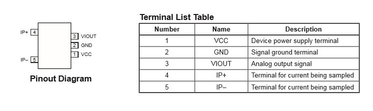
We measured the current from our motor voltage source using a Hall Effect Current Sensor. The datasheet for the sensor we used can be downloaded from here under the datasheets tab on the side, here's the pin diagram of the sensor taken from the datasheet:
The input voltage to the motor is measured by connecting a wire parallel to the positive terminal of the power supply, which is then put through a 1:3 voltage divider made up of high resistance resistors, with the output being a quarter of the input voltage. This is to protect the MCU if we decide to run the motor as high as 12V. The output is then measured by the ADC, and calculation is done to reverse the voltage divider to get the voltage that the motor is acutally seeing.
To get voltage, current sensor and strain gage to work together, we needed 3 ADC channels. However, the conventional method with muxes only allows up to 2. Thus we had to switch ADC to SCAN mode, and read the scanned results in buffers 0, 1 and 2 for the 3 ADC results.
To measure the rate of the motor, we used a photo interrupter, an infrared light sensor that can detect when an object passes between two uprights. One of the uprights on the sensor contains an infrared emitter and the other contains an infrared emitter.
To initially test if the sensor works, we supplied 5 V to the sensor and wired it to the oscilloscope. When the gate of the sensor is clear, the oscilloscope showed a straight line at approximately 5 V. When something obstructs the gate, the signal drops to approximately 0 V. Once we tested this, we mounted the sensor onto the mechanical setup so that every time the motor rotates, we can measure it’s frequency and thus, the RPM.
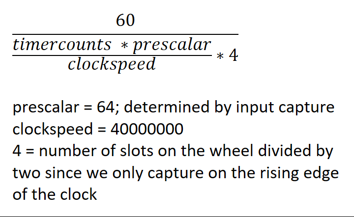
To periodically read the sensor, we have an interrupt service routine that reads the input capture at the rising edge of the clock. This means that for every rotation the sensor outputs either 5 V or 0 V which is then read by the input capture. The setup for this is: OpenCapture4( IC_RISE_EDGE | IC_INT_4CAPTURE | IC_TIMER3_SRC | IC_ON ) and ConfigIntCapture4(IC_INT_ON | IC_INT_PRIOR_3 | IC_INT_SUB_PRIOR_3 ). This sets up the time capture and turns on the interrupt so that every capture can be recorded. In the PID thread, if the timeCapture is equal to 0, we set the timeCapture to 1 (to later avoid a divide by 0) and continuously calculate the raw RPM with the following equation:
Plugging in the values into the equation, we get 9375000. We then divide that by the time capture to get the final, raw RPM value. Then, we applied an IIR filter by initializing a variable, rpm_filt to zero, calculating the difference of the raw rpm value and previous rpm value, dividing that by 16 and adding it to rpm_filt. This filter was initially added to help stabilize RPM values, but we used the raw rpm values for our control mechanism at the end because we found that the raw rpm values matched the tuned system better.
The DC input power is simply V*A, which can be found by multiplying the measured voltage with current. However, the mechanical output power is more complicated. Rotational mechanical power is defined as torque multiplied by the angular velocity, in units of radians per second. So we had to convert the measured RPM to rads/sec and multiply that by the torque in N-m to get at power in Watts.
To get efficiency, we took the output power and divided it by the input power. It is multiplied by 100 for display in percent.
Servo controls were simple but tricky to figure out at first. They basically have their own control system inside that reads a PWM high-pulse anywhere between 1-2ms (on the white signal line, red for power and black is common ground), and sends the servo to maintain the proportional angle. So if we send a 1ms pulse, the servo goes to its minimum position, and 2ms it goes to the max. We used digital servos which responded faster than analog ones, and were more precise in its maneuvers.
We originally had a motor controller for the DC motor that malfunctioned, so we just varied the voltage on the high-current supply for control. However,the control for that is very much the same as the servo controls; 1.5ms duty cycle for neutral, and 2ms for full forward power. In the future, we would not be able to directly drive a brushless motor off a power supply, so this would be very useful for our custom motor controller(we kept the code).
To save our data, we chose UART to serially communicate between the PIC32 and the computer. We used a UART to USB serial cable, and the transmit/receive setup from this protothreads example. All we needed to do was transmit rpm and voltage from the PIC32 to the computer, so we instantiated pt_input, pt_output, pt_DMA_output for UART control. These threads are written and spawned from pt_cornell_1_2_2 and config_1_2_2 every time we want to send information. These files also set up the UART and DMA pins and initializations. To send information, we store our message to the PT_send_buffer buffer and then call PT_SPAWN on pt_DMA_output and PT_DMA_PutSerialBuffer.
On the computer, we use Putty to both view and log our data. Every time we run the system and have Putty open, the data is auto-saved and can be used by going to PuTTY -> PuTTY Configuration -> Session -> Logging. In Logging, locate or create a directory to save the data, and give a file name. We use "&H-&Y&M&D-&T.log" in our final project folder so that a new file is created everytime. Note that if you choose a specific file name (i.e "testfile.log"), the data will either be overwritten or appended to previously collected data. Alternatively, you can choose "Ask the user every time". Then, click on Session -> Default Settings -> Save to make this logging format your default setting.
Upon reset, the system will begin runing our preprogrammed test sequence. The test sequence uses the first 120 seconds for calibration of the strain gauges and digital potentiometer; during this period the servos remain opened and sensor data is not sent over UART. Next the system must measure the no load RPM resulting from the selected voltage level. After the no load RPM is measured, then the program begins breaking (using the servos) to reach different percentages of the RPM. The torque, RPM, and calculated efficiency at these designated RPMs are then saved and transmitted. In our test sequence, the measured RPMS are: no load, 95%, 90%, 85%, 80%, 75%, 70%, 65%, 60%, and 55%. We initially wanted to take data by decresing the percentage by 10%, however, we found that if the RPM got too low, then the servo would immediately stop the rotating shaft and the system would stall since RPM could not get any lower. Between each of the data collection states, we pause transmission and allow the servos time to break to reach the desired RPM. This increases the accuracy of our measurements for torque, which is a running average, by eliminating values corresponding to undesired RPMS. After the 55% of no load RPM measurements are complete, the sequence returns to wait for five seconds before repeating the loop. The repetition of the entire test sequence did not work during testing; we found that the servos would open correctly but then close completely. To get new data, we had to reset the system.
The test sequence was implemented into our code as a state machine based on the variable rpm_state with 12 states: ten corresponding to the ten measured RPMs mentioned above, one called PREP where the servos engage until they reach the desired RPM, and one called WAIT which accounts for the initial calibration time and lets the user change the voltage in between trials. The ten RPM level states are named NOLOAD for no load rpm, NINETY for 95% of no load, EIGHTY for 90%, SEVENTY for 85%, SIXTY for 80%, FIFTY for 75%, FORTY for 70%, THIRTY for 65%, TWENTY for 60%, and TEN for 55%
The system begins in the case WAIT. WAIT first evaluates a conditional that checks if the overall system run time (stored in variable tm) is between 100 and 120 seconds and prints "starting" on the TFT; this serves as a warning for the end of the calibration period and lets the user know they can begin increasing the supplied voltage. We want to increase the voltage later in the calibration period because during calibration it is better to supply no or low voltage to the motor to prevent the mechanical set up from vibrating excessively. Next in WAIT is an if-elseif-else branch that does the following. First it checks if tm is greater than the 120 sec calibration time and whether a variable cont is 0, if the condition is true then we know to begin the test sequence. To begin, it sets the rpm_state to PREP, the destination state (stored in the variable dest) to NOLOAD, rpm_des to rpm_sum (initialized to zero), time to PT_GET_TIME(), cont to 1, and opens the servos. The condition for the else-if branch is to wait for 5 sec have elapsed after the end of the first sequence and check if cont is 1. The else-if does the same as the if statement, but is executed after one sequence is complete. If either condition fails, the else statement simply keeps the rpm_state at WAIT.
The PREP state allows the system to attain the specified rpm in rpm_des prior to recording data. It also contains an if-elseif-else branch which does the following. First in the event that we have begun a new sequence and the destination state is NOLOAD, then we change rpm_state to dest, clear the running sum for torque (run_sum), set the running sum for RPM (rpm_sum) to newtime (the RPM measured from the photointerrupter), the number of data points collected to 1, and the time to PT_GET_TIME(). If the destination is not NOLOAD, then the next condition in PREP checks if the current rpm in newtime is greater than the desired rpm. If newtime is greater, than the shaft is spinning too fast and we want to engage the servos to slow down RPM. This is done by increasing des_angle1 and des_angle2 gradually (by increments of 10) and writing those values to the servo PWM until the else-if condition is false. Once the desired rpm is attained, then the program enters the else branch which clears run_sum and num_points and updates time and rpm_state to dest.
The rest of the RPM states follow the same structure. The system remains in each of the RPM states for four seconds. During the four seconds, data is collected in the else statement which updates the running sums for torque (run_sum) as well as the number of points collected. If four seconds have elapsed, then the running average for torque and the desired rpm are transmitted through UART to a PC. Additionally, rpm_des is decremented to the next percentage of the no load RPM and the destination state is set to the corresponding state (unless we are already in the lowest rpm state (55%) in which case the destination is set to WAIT); we also send the program to PREP to engage the servos. NOLOAD is a special case in that here we also calculate the running average for RPM and store the value in rpm_sum; this is the no load RPM used as a reference for the rest of the states to calculate rpm_des.
For our final demo, the collected data was the following:
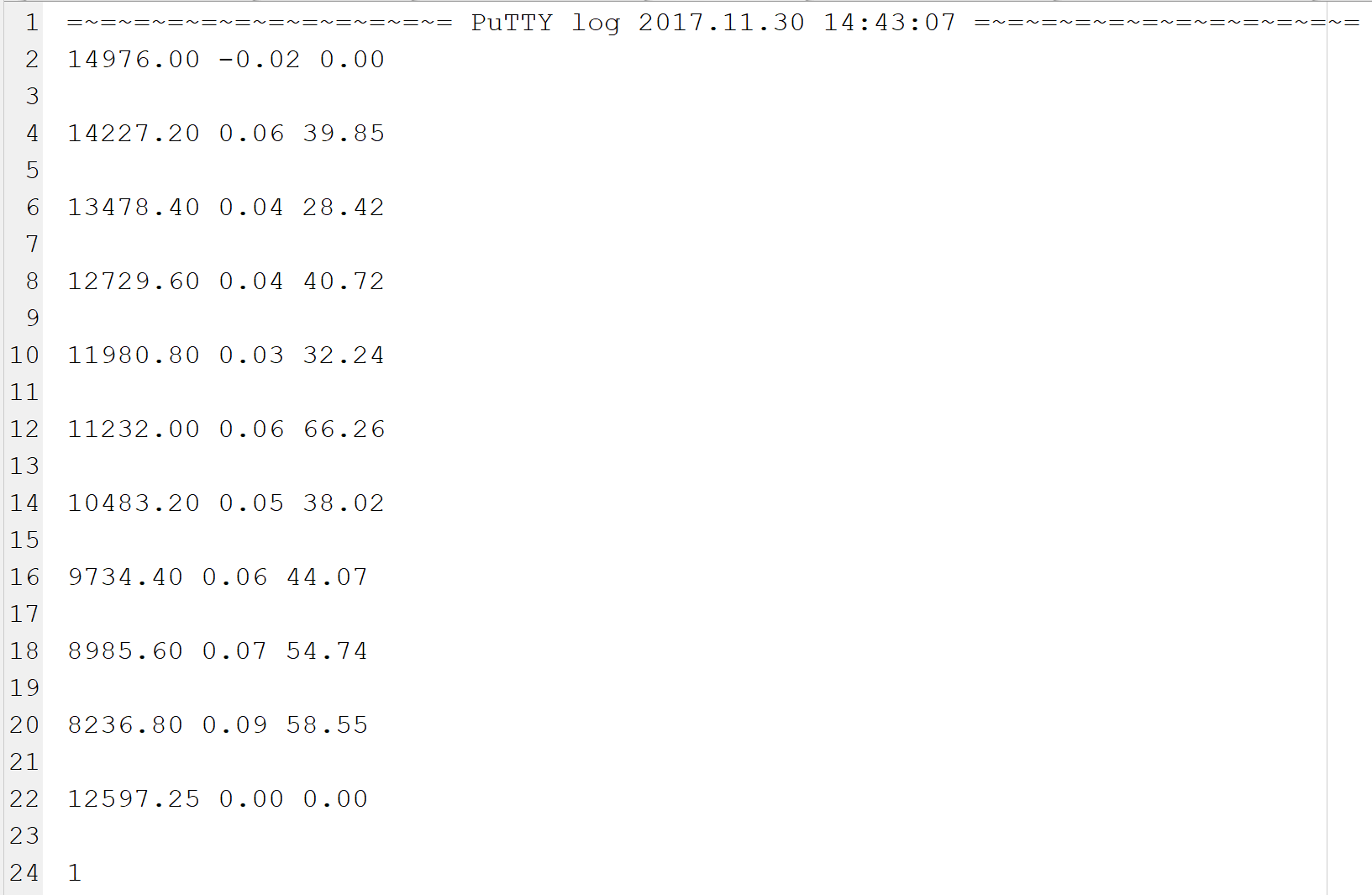
In this text file, the first line is the header, every other line is empty and the last line was cut off when the data collection was stopped. The parsing method described above handles these issues, and then produces the following contour map:
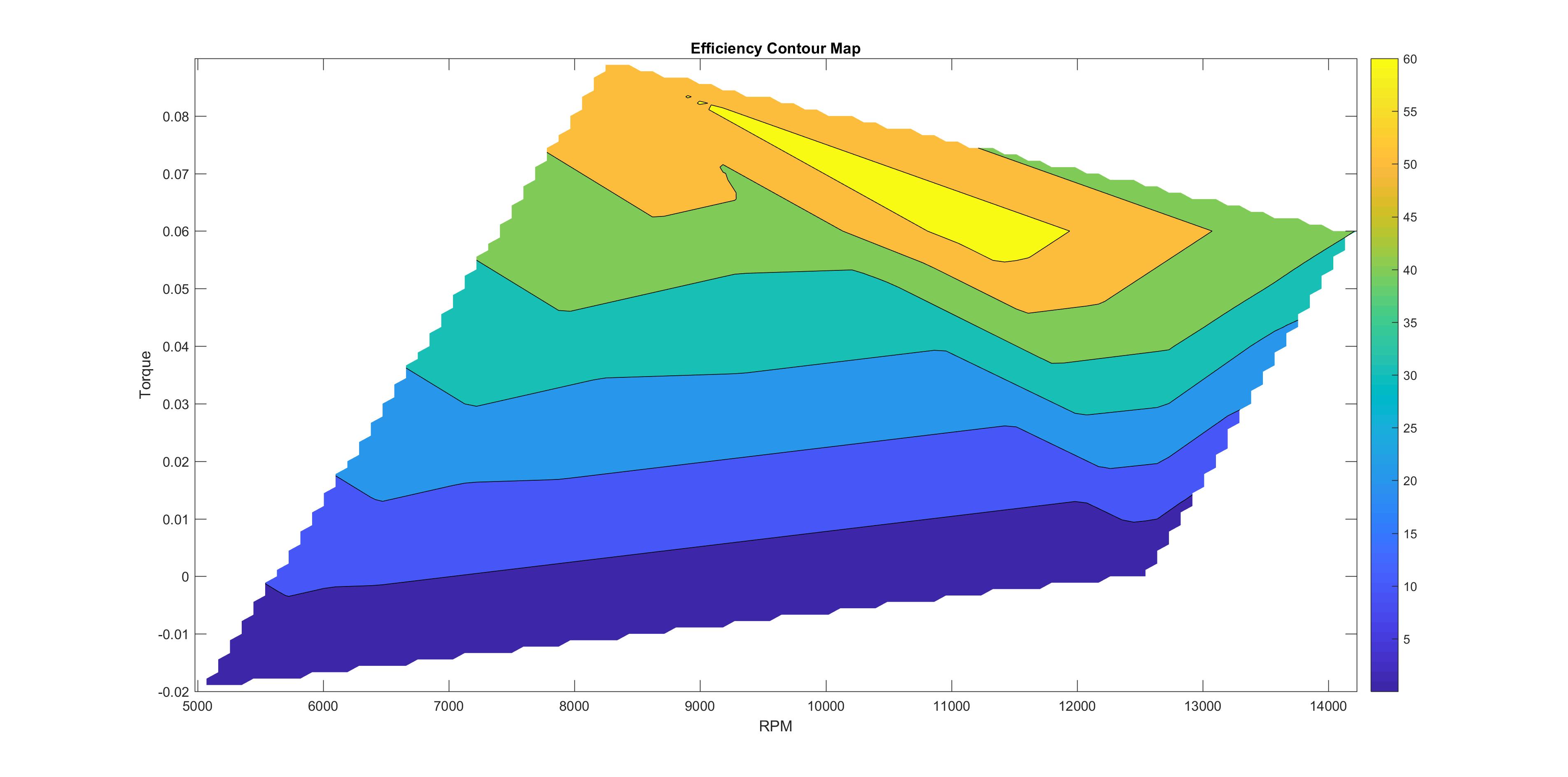
Here, we can see that at peak efficiency can be observed within 10000 – 11000 RPM and 0.05 – 0.07 N.m of torque. We only took a few data points here, so a more systematic sweep would produce better results.
One trade-off that limited the speed of execution of our system was the accuracy of the readings taken. Since accuracy is a higher priority than fast execution, we made changes that slowed down our testing sequence in favor of more accurate data. For example, in the final version of our dynamometer code, the test sequence allows for 120 seconds of calibration instead of the previous 45 seconds. This change gives the digital potentiometer nearly three times the time to zero out and balance the wheatstone bridge we get our torque measurments from. The extra time also lets the user give lower voltages to the motor during calibration instead of having to immediately turn up the voltage to that desired for testing, lowering the effect of vibration on calibration.
Additionally, the test sequence increments the servos PWM value by only 10 values at a time. We chose this value because we found that incrementing one was by far too slow, yet increasing this value to say 100 decreased the accuracy as the RPM would decrease too rapidly.
Due to the fact that we decided to test the system with a small brushed DC motor, the early test results do not appear to be very accurate. The magnitude of torque we expect to measure is on the order of 2-5 N-m, whereas the brushed motor is only capable of exerting 0.1-0.2 N-m at best. Therefore, the results vary and could be seen in the test run video. However, we expect this to be a lot better once we move on to test the larger brushless DC outrunner motors, which was the purpose for this project.
To keep our design safe, we constructed a shield for the main body out of plexiglass. During operation the shield is placed in front of the main mechanical setup to block any material that may fly off. Another safety concern we faced in our design was the danger of using high power. To address this issue, we compartmentalized the components of our system that would be carrying high current and/or high voltage to protect the other parts of our system. Additionally, we used wires with more insulation for our high current wiring and wrapped any exposed sections at connections with shrink wraps and/or electrical tape.
No significant interference problems were observed throughout this project, since no signals were transmitted wirelessly.
Looking back our expectations, the results of what we were able to accomplish exceeded our expectations for the class project: all sensors worked and were integrated together, the test sequence is nearly completely autonmous, and based on the contour maps we have seen from our few trials, the data collected seems reasonable and will be useful for future use by the Resistance Racing team. Further work we could do to improve our project even more is to have the test sequence able to loop back after changing the voltage supply. This way multiple trials can be run and stored on the same text file rather; as of now, the data from different trials must be manually concatenated in order to display all collected data on the same contour map. This can also be improved with the integration of the motor controller for the brushless system, since that way with a more complex sequence we would be able to do sweep with a large number of data points.
In addition, data processing in the microcontroller system can be improved, by playing around with different filters and zeroing algorithms. Using a better powersupply would also help with the data collection, since we were getting some inconsistent results due to noise in testing.
We must say a big thank you to Professor Land for believing in us and this project, even when other professors and lab technicians were telling us this was not possible.
The sources we used for inspiration and help were mainly public forums or programming sites such as matworks. We did base some of our code off of the examples provided on the ECE 4760 course website and looked at tutorials for how to go about using our strain gauges and current sensor. We cited all references used in Appendix F.
During this project, we tried to maintain and follow the IEEE Code of Ethics by ensuring the safety of our project and seeking help from others. Due to the complexity of our mechanical system, one of main priorities was keeping the system safe. We built our system in a bottom-up fashion, integrating smaller modules together until everything was connected; as we did so, we continually added safety features that addressed potential dangers. For example, once we integrated the high power supplies into our system, we changed our wiring to keep high power sections separate and added wires designed to handle high current and high voltage to these subsystems. Additionally, we created a plastic shield for the rotating section of the mechanical setup.
Since we completed this project in collaboration with the Resistance Racing project team, we made sure to inform both Professor Bruce Land and Resistance Racing advisor Professor Joe Skovira of our intentions prior to beginning this project to avoid any potential conflicts of interest. Throughout this project, and course as well, we sought honest criticism of our ideas and advice from Professor Land and the teaching assistants of this course and other faculty in the Enginnering school including Professor Alan Zehnder and Liran Gazit. Additionally, we pulled information and inspiration from online and credited them in text and Appendix F of this document.
Lastly, we strove to report the results of our project in a honest and clear manner. The data we collected came directly from the sensors integrated in our system. The contour map was used to display the data in a meaningful way.
The group approves this report for inclusion on the course website.
The group approves the video for inclusion on the course youtube channel.
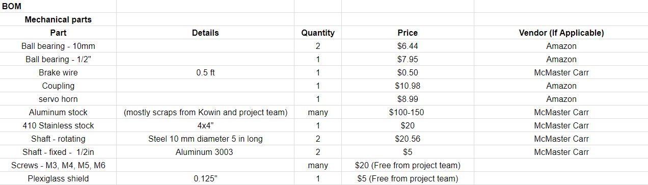
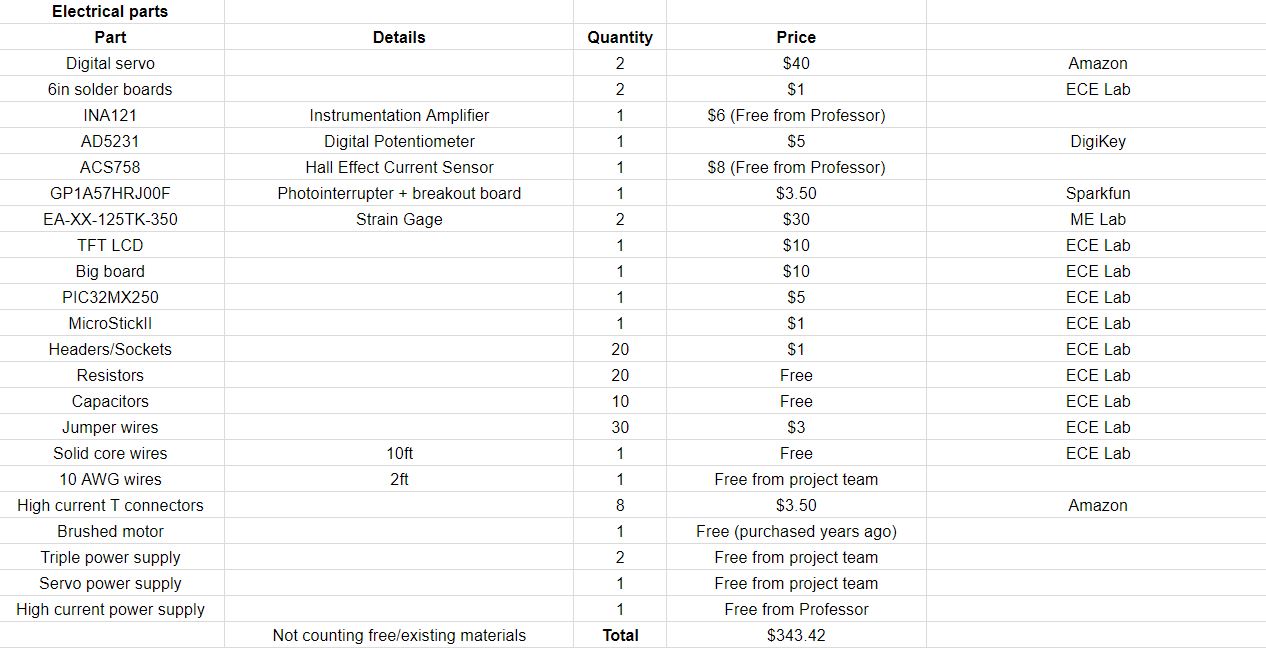
Since this was done as a part of the Resistance Racing project team, most of the costs were handled by the team. And so the budget limit was removed as explained in the lab 5 webpage.
Tasks worked on by Aasta Gandhi: UART communication, current sensor calibration, contour map MATLAB code, test sequence code, photointerrupter/RPM code, code integration, wheatstone bridge/amplifier circuitry
Tasks worked on by Kowin Shi: design and manufacturing of mechanical setup, strain gauge mounting, software filters for sensors, high power wiring, digital potentiometer calibration code, wheatstone bridge/amplifier circuitry
Tasks worked on by Erika Yu: current sensor calibration, contour map MATLAB code, test sequence code, soldering of power rail circuitry, high power wiring, wheatstone bridge/amplifier circuitry