ECE 476 Final Project:
A Microcontroller Based Turbidity Meter
By: Jesse Adland (jsa25@cornell.edu)
and Jay Huang (jyh25@cornell.edu)
Introduction
A Low-Cost Turbidity
Meter for Underdeveloped Countries
Our project is a collaboration with an independent research
project being conducted by senior civil and environmental engineering student
Background
What is Turbidity?
According
to the Environmental Protection Agency (EPA), turbidity is:
The cloudy
appearance of water caused by the presence of suspended and colloidal matter.
In the waterworks field, a turbidity measurement is used to indicate the
clarity of water. Technically, turbidity is an optical property of the water
based on the amount of light reflected by suspended particles. Turbidity cannot
be directly equated to suspended solids because white particles reflect more
light than dark-colored particles and many small particles will reflect more
light than an equivalent large particle.[1]
Basically,
this means that turbidity is closely related to the amount of light scattered
at 90 degrees when a light source is shined through a sample. Our measurement process takes advantage of
the relationship between optical scattering and turbidity to take measurements
of the turbidity of liquid samples.
How Do We Measure Turbidity?
When
particles are suspended in water and a light is shined through the sample, not
all of the light will pass straight through the sample. Instead, the light will reflect off of the
suspended particles and some of the light will exit at a right angle to the
direction of entry into the sample. Our
meter uses a laser pointer as a light source, and two photodiodes as detectors
for the intensity of the transmitted and refracted light. The basic setup is shown below in figure 1.
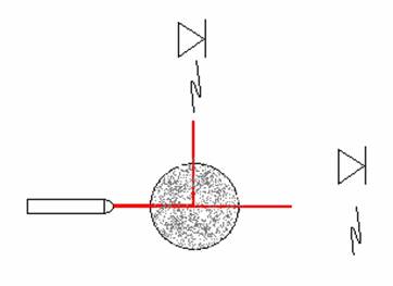
Figure 1: schematic
concept of turbidity meter.
By
measuring the voltages off of both of the photo diodes, we can derive a
function which calculates turbidity from the ratio of the voltage across the 90
degree sensor to the voltage across the 180 degree sensor.
In
order to prove that our idea was sound, we used equipment in one of the civil
and environmental engineering labs to test out the design. We mixed kaolin clay and water to create
samples of varying turbidity. We measured
the samples on a calibrated turbidity meter, and then took measurements from
our device. The results are shown
graphically below in figure 2.
Figure 2: Turbidity vs
Voltage Ratio
It is
apparent that there is some function which will define the turbidity of a
sample as a function of the voltage ratio from the sensors. As it turns out, a quadratic least squares
regression line is a very close fit to the data.
Calibration Standards
The
EPA sets the calibration standard for a turbidity meter quite high. The following are the EPA for turbidity
meters:
The sensitivity of the
instrument should permit detection of a turbidity difference of 0.02 NTU or
less in waters having turbidities less than 1 unit. The instrument should
measure from 0 to 40 units turbidity. Several ranges may be necessary to obtain
both adequate coverage and sufficient sensitivity for low turbidities.[1]
These
standards are probably beyond the capabilities of the sensors that we chose and
the ability of the microcontroller to process.
However, the point of this project is not to create a perfect meter, but
rather a viable low cost alternative.
Despite the fact that our resolution does not necessarily live up to EPA
standards, the meter can still be quite useful in a laboratory setting.
Getting Samples to Measure
The
principle of turbidity measurements was described in the above section. In practice, taking these measurements turned
out to be far more difficult than was imagined.
The first large problem that we encountered was the quality of the
samples which we were attempting to use to calibrate the meter with. Because we had to work on our project in the
476 lab space, we needed to get samples of known turbidities which were
contained in glass cuvettes which we could bring into the lab. We measured the turbidity of our samples in a
calibrated turbidity meter in a civil and environmental engineering
laboratory. The standard sample which is
used to calibrate turbidity meters is formazin in water. However, formazin is a carcinogen and
expensive, so we looked for alternative materials use.
Kaolin
clay mixed with water was the first sample type which we tried. The downfall of Kaolin clay is that is does
not form a homogeneous solution with water, and it settles out over time. This means that while the sample is in the
meter, small chunks of the clay will float between the photodiode and the
laser. This results in unstable
measurements of turbidity even on a calibrated piece of laboratory
equipment!!
Our
next attempt at finding stable samples also went sour. Regular 2% milk does form a homogeneous
solution in water. We mixed milk with
water to create samples of various turbidities, all of which were stable. However, milk is an organic substance which
means that is spoils over time. Despite
our best refrigeration efforts, after one night, the sample went bad and the
turbidity changed.
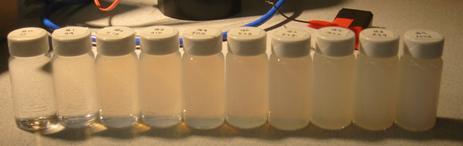
Figure 3: Hydrophilic Cutting Oil in Disposable Glass
Cuvettes
Our final effort was clearly the best. We diluted a hydrophilic cutting oil into water to make stable, homogeneous, non-organic samples which do not settle out over time. The samples are shown above in figure 3. The turbidity remained stable over a period of several days (and counting…).
Hardware
Design
Housing the Sensors
Mixed
in with the process of discovering the importance of stable samples was
learning the importance of a stable receptacle for those samples. The original design for the turbidity meter
was created by James Berg out of foam core cardboard. This setup is shown below in figure 4. Eventually, after much frustration, we
discovered that when we put samples into the cardboard, the housing of the
meter flexed, and the alignment of the laser to the photodiodes changed by as
much as 10% in either direction.
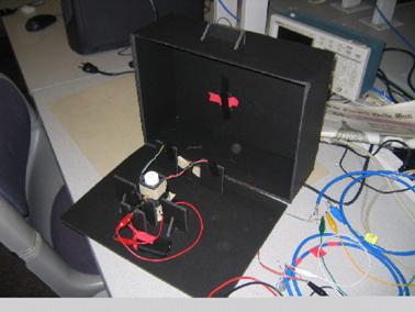
Figure 4: Foam Core
Container for Turbidity Meter
In
order to try to minimize the movement of the sensors, light source and sample,
James created a hard nylon container for the meter. This container is shown below in figure
5. There are holes drilled into the
sides for the photodiodes and the laser pointer. The precise machining keeps the sensors from
moving with respect to the light source.
However, the diameter of the hole for the cuvettes was slightly too
large. The results was that the
placement of the cuvette in the holder could drastically adjust the readings on
the sensors. Because the laser is a
highly correlated and directed light source, the angle at which the beam hits
the glass changes the amount of light which is reflected and transmitted. In order to combat this, we found a new,
disposable cuvette (the ones shown in figure 3) which was slightly larger in
diameter. James machined the nylon
holder to within 1/1000 inch precision.
The cuvettes cannot move with respect to the laser, and the readings are
very steady.
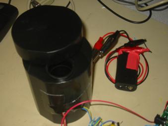
Figure 5: Black Nylon
Container for the Meter
After
moving to the black nylon container, we also decided to focus on the entire
range of turbidity (0-1000 NTU) rather than just the range 0-50 NTU. We had been focusing on increasing the
resolution in the low range, but we decided that a more reasonable goal for
this project was to try to get good (not great) readings across the entire
scale. Although we have not had the
opportunity to test the resolution of the new housing for sample in the range
0-50 NTU, we have high hopes that the new housing will also improve resolution
in this range.
From Photodiodes to the MCU
After
receiving James’ measurements (shown in figure 2), we realized that one of the
main challenges of this project would be taking input from the photodiodes to
the ADC. The ADC on the on the
AtmelMega32 MCU has 10 bits of resolution, or 1024 distinct levels, between GND
and Vcc. In the range from 0-50 NTU the
voltage across the 90 degree sensor varies from .0633V to .1477V. Without amplification, that corresponds to
(.1477V-.0633V) * 1024levels / 5V= 17 levels.
This means that we need to
amplify the voltages from the sensors so that they resolve to as many different
levels as possible. If we use a
non-inverting amplifier, such as the once shown in figure 6, we can get a gain
of up to 30 without clipping the input.
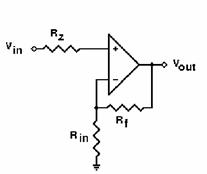
Figure 6: Non-Inverting Amplifier Circuit Gain=
(1+Rf/Rin)
By using the circuit shown in figure 6, we can get a maximum
resolution of (.1477-.0633)* 1024 levels/ 5V *30 = 518 levels. This is enough resolution to divide the range
of 0-50 NTU into the desired 500 levels.
However, we can actually still attempt to further increase the
resolution. The voltages on the 180
degree sensor vary from .5472V to .5196.
With the schematic shown in fig 6, we can only chose a gain of 8 before
we begin clipping the input signal.
However, by using a differential amplifier we can subtract off a constant
bias voltage and then multiply the difference by a constant gain. The schematic
shown in figure 7 allows us to implement this amplifier.
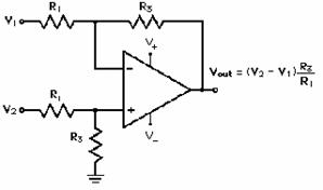
Figure 7: Non-Inverting Differential Amplifier
We chose a bias voltage of .5 V for the 180 degree
sensor. The gain we chose was R3/R1=
150. This allows to resolve the 180
degree sensor into (.5472-.5296)*150*1024/5V = 845 levels. This was more than enough for the required
resolution.
However, as it turns out, nothing which was just discussed
is actually included in our final project.
Although we spent a lot of time creating these amplifiers, when we changed
to the black nylon housing, the sensors began picking up a larger portion of
the laser light. The swing in voltages
was much larger than the data we originally planned on. We ended up only using the non-inverting
amplifier (figure 6) implemented with a LM 358 dual op amp. We chose a gain of 5. This sufficed to read the sensors accurately.
Software Design
The software backbone is a state machine (see Overall State
Diagram in Appendix) running off several timers. There are a total of five timers
counting in ms, each of which is reset to zero according to different
conditions. time1 counts to 5 ms, dictating the frequency at which the ADC
registers are read. Because there is more than one ADC input (two in the final
design), alternating between inputs in an orderly manner is necessary. time2
counts to 3 s, after which all completed states return to the “wait” state
displaying the default “Ready.” message on the LCD. time3 controls the LED to
flash during recording mode. This allows to user to know at a glance if
recording is completed without having to read the LCD output. time4 debounces
the increment and decrement buttons every 120 ms. This period is reasonably
larger than the usual 30 ms used in button debounce because the button state
machine implements two scales of increment or decrement according to the
duration of the button hold. Also, the buttons used are different from the
usual lab push buttons. time5 counts how long the button is held in the button
state machine.
The trickiest part about writing the program is putting the
states of the overall state machine together. The best way to describe the
state machine is to outline how a user operates the project. The moment power
is turned on, the machine stays in the “wait” state. States that return to the
“wait” state have their final LCD messages staying on screen for 3 s before the
default “Ready.” message appears again. Pressing the “Record” and “Calibrate”
buttons take the user to the respective states. The user can press “Cancel” to
return to the “wait” state, nullifying any readings or calibrations. However,
if the user is already in the “wait” state, the “Cancel” button displays the
regression coefficients. This was implemented as a handy debugging tool. In the
“Record” state, the ADCH and ADCL registers are both read to obtain 10 bits of
accuracy. The ADMUX register is appropriately set to use AVcc as the reference
voltage as well as alternating between the two analog inputs from the 90 and
180 degree photodiodes. Because five thousand of each ADC reading is taken for
each sample, the noise fluctuations are virtually eliminated after averaging.
The average ADC readings from the 90 degree and 180 degree inputs are used to
compute their ratio, which is used in the regression equation to obtain the
corresponding NTU value. This value is displayed on the LCD and the machine
returns to “wait”. Also for debugging purposes, the normalized ratio is
displayed. The normalization is discussed below.
In the “Calibrate” state, the machine is sent to the
“Record” state to obtain a certain number of calibration data readings, the
default being eight data points. After each calibration reading, the machine
goes to the “Input” state instead of calculating and displaying the NTU reading
as before. In the “Input” state, the user adjusts the NTU reading as shown on
screen to the desired calibration value. This adjustment uses the button state
machine (see Button State Diagram in Appendix). In all these transitions, the
“Record” button is used as a “Confirm” button. The button state machine allows
for increments and decrements in two ranges for the convenience of the user. A
button tap corresponds to +-1 NTU while a hold causes a rolling +-10 NTU. After
the input is confirmed, the machine goes back to “Calibrate”. If necessary, it
transitions to “Record” to obtain more calibration values. Otherwise, least
mean square regression is calculated for the ratio and NTU data points. The end
result is three coefficients for an order two regression curve, where the input
is the ratio and the output is the NTU. The regression coefficients are stored
permanently in EEPROM, so each turbidity meter only needs to be calibrated
during the first use.
Our initial goal was to use two regression curves to
calculate the turbidity of the samples from two sets of different analog
amplifications. The plot of NTU value against reflected/transmitted ratio
showed that smaller NTU values could benefit with higher turbidity resolution
if they used greater amplification and a separate regression curve from the
larger NTU values. To achieve this, the software was initially written to
accommodate readings from four analog inputs (PINA.0 to PINA.3), and
correspondingly, two ratios from differently amplified inputs. Also, code was
written to obtain a second regression curve. After taking readings from any
particular sample, the software decides whether to use the low range or high
range regression curve based on the calculated turbidity value. For example, a
turbid sample would have a high ratio beyond a certain threshold, and the
program would choose the high range regression coefficients to calculate the
turbidity. Unfortunately, as previously mentioned, the photodiodes exhibited
too much fluctuation using the first housing design and ultimately resulted in
our decision renders to operate on a single large range. Thus, the final
version of the software only implements one pair of ADC readings, one ratio and
one regression curve.
An interesting phenomenon we noticed was that the MCU
exhibited different arithmetic precision for floating point operations in
different ranges of numerical values. Floating point multiplications and
divisions involving numbers much smaller than one severely deviated from
expected results. Surprisingly, scaling those small numbers by a constant
factor into the range between one and ten greatly improved the accuracy.
Because the measured ratios are all smaller than one, we subtracted a constant of
.5 from each and scaled the result by ten to put them between one and ten. This
method greatly improved the accuracy of the calculated regression coefficients.
The code in this project was written entirely by us, with reference to ECE 476 lecture material.
Results
Because 3000 ADC readings are taken in intervals of 5 ms, our
meter gives a NTU value in 15 s. In comparison, a commercial turbidity meter
gives a stable NTU reading between 15 and 30 s. To rigorously prove the
accuracy of our meter, we conducted many trials to compare the turbidity of
samples measured with a commercial meter against values calculated with our
meter. The following table shows a typical run with nine samples with turbidity
ranging from 99 to 1005 NTU. The voltage readings off the 90 and 180 degree photodiodes
are measured, and their ratios are calculated. The final column of the table
shows the calculated turbidity from our meter using the second order regression
equation.
Table 1: Voltages,
Ratios and Calculated Turbidities
|
Sample |
Measured NTU |
90 Degree Photodiode |
180 Degree Photodiode |
Voltage Ratio |
Calculated NTU |
|
1 |
99 |
0.067 |
0.315 |
0.212698 |
97.3922 |
|
2 |
216 |
0.133 |
0.309 |
0.430421 |
200.7855 |
|
3 |
315 |
0.164 |
0.306 |
0.535948 |
365.3601 |
|
4 |
405 |
0.178 |
0.320 |
0.556250 |
405.5945 |
|
5 |
523 |
0.192 |
0.314 |
0.611465 |
529.0092 |
|
6 |
627 |
0.197 |
0.304 |
0.648026 |
621.9892 |
|
7 |
722 |
0.202 |
0.304 |
0.664474 |
666.7424 |
|
8 |
899 |
0.210 |
0.284 |
0.739437 |
893.7093 |
|
9 |
1005 |
0.212 |
0.272 |
0.779412 |
1030.1600 |
A regression curve is also plotted for the above data. Here, the R2 value of 0.9913 indicates a good fit of data to curve, where R2 = 1 represents a theoretically perfect fit.
Figure 8: Turbidity as a Function of Voltage Ratio
As can be observed from both the table and the plot, the turbidity measured with our meter is mostly in the ballpark of the actual measured turbidity. Even though our meter cannot always guarantee the correct turbidity or any fixed accuracy, our project proved that the concept of using reflected/transmitted light voltage ratios to calculate turbidity is feasible and robust enough to operate over a reasonably large turbidity range.
Conclusions
While our final version of the project works reasonably well over the range 0-1000 NTU, we were not successful in creating a device which can accurately measure turbidity with high resolution between 0-50 NTU. We did not get a chance to try the final version in this range, and hopefully we will see the same consistent results at lower turbidities that we did at higher values.
Some of the problems we encountered could possibly be resolved by making simple changes in the hardware. For example we had problems with reflections off of the glass cuvettes from the laser. A non-correlated light source would minimize the effect of these reflections. Also, the photodiodes which we chose are tuned for maximum response in the infrared region. We used a red laser. We could either choose a light source in the infrared or chose more appropriate sensors.
As electrical engineers, we must always work with the IEEE code of ethics in mind. In the context of our project, several important points applied. First, we recognize that our meter can be used in situation where failure can be harmful to human health. Water quality measurements must be accurate. We attempted to design a device that gives consistent, accurate readings and will not fail. However, when our design failed to reach the appropriate calibration standards, we were sure to honestly disclose that information. Although we were not offered any bribes, we would not have accepted them had they been offered. During the design process, we often sought the opinions of teachers and teaching assistants on the viability of our project. Also, we attempted through the spirit of collaboration to help our colleague James advance his professional career.
Appendix A – Commented Code
Appendix B – Schematics
Implementation
Flow Chart


Appendix C – Parts List and Budget
|
Part
Name |
Quantity |
Price
($) |
|
|
|
|
|
White
Board |
1 |
6 |
|
Custom PC
Board |
1 |
5 |
|
Mega32 |
1 |
8 |
|
LCD
(16x2) |
1 |
8 |
|
LM 358
Dual Op Amp |
1 |
1.04 |
|
9V |
1 |
4 |
|
Chunk
Black Nylon |
1 |
found |
|
Laser
Pointer |
1 |
found |
|
OPF470
Photodiodes |
2 |
found |
|
Push
Buttons |
5 |
found |
|
|
|
|
|
|
|
|
|
Total
Price |
|
$32.04 |
Appendix D – Team Members Actions
Jesse-
1) Researched Background on Turbidity
2) Wrote algorithm for quadratic least squares regression
3) Extensively tested various project versions
4) Mixed samples of milk and water
5) Mixed samples of oil and water
6) Wrote hardware portion of report
Jay-
1) Wrote overall state machine for project
2) Extensively tested various project versions
3) Built non-inverting amplifiers
4) Mixed samples of oil and water
5) Wrote software portion of report
6) Wrote results section in report
Appendix E – References
2) LM 358 Dual Op Amp Datasheet
3) OPF470 Fiber Optic PIN Photodiode Datasheet