Introduction
Back to TopThe Music Wand is a device that optically reads printed sheet music in real-time and synthesizes the notes which are read from the page.
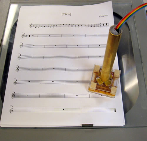
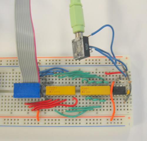
The device uses a linear image sensor mounted on the end of a handheld wand to scan printed sheet music and identify the note pitches. For each note detected, a synthesized piano note is played at the detected pitch. We chose this project in order to explore image processing and sound synthesis on the microcontroller in a creative and practical context. The concept of a music-reading wand appealed to us because it would allow a novice musician to easily learn sheet music without the help of a musical instrument.
The Music Wand was developed and built as a design project for ECE 4760 in the Cornell University School of Electrical and Computer Engineering.
High-Level Design
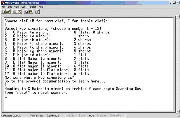
Back to TopDue to the performance limitations of the microcontroller, sophisticated image processing on the microcontroller is very difficult and thus is not often attempted. In order to get around some of the problems of image processing, we chose the well-defined application of reading music. This allowed us to significantly decrease the amount of computation required by the microcontroller by taking advantage of the nature of musical notation. The key to the success of our project was the structure of the musical staff, where the five parallel staff lines gave us a basis for orientation and note recognition. In addition to the image processing algorithm, we designed a user interface from the PC to the MCU via serial port (using Windows Hyperterminal) with which the user selects the clef and key signature of the music to be scanned. During scanning, the notes detected by the image algorithm are played using an enhanced version of the Direct Digital Synthesis (DDS) scheme presented to us earlier in the year.
Background Math
Direct Digital Synthesis (DDS)
Direct Digital Synthesis is implemented similar to the method used in lab 2, with some modifications. The basic operation is the same. We still use the fast PWM mode on the Mega32's timer 0, an accumulator table, a 256 entry sine table, and an increment for the accumulator based on the desired frequency. To improve accuracy, we use a 32 bit accumulator and a 32 bit increment. Since the sine table has 256 entries, we only use the upper 8 bits as a lookup index into the sine table, which holds 8 bit chars. Once again, the maximum frequency we could generate was about 3.9KHz with 16 samples per wave. Instead of using the internal DAC through OC0, we decided to create an external DAC for accuracy (see Hardware Design).
|------------------------------------------------32 bits-----------------------------------------------------------|
8 bits for sine table |
24 bits to increase resolution |
Sample Accumulator Table. The increment is added to this table at each cycle of the PWM.
Notice that only the top 8 bits are used to retrieve a value from the sine table. As we will see in the following calculations, the resolution of the DDS is set by the number of bits in the accumulator, thus we used 32 bits instead of just the minimum of 8.
The required increment for each frequency was calculated using the following formulas:
(1) Fs=clk/N
This formula relates the sampling frequency of the sine wave Fs to the clock speed on the mega32. In fast PWM mode, N=256, giving Fs=16MHz/256=62.5KHz. This means that we can sample the sine wave at a maximum rate of 62.5KHz.
(2) Resolution=Fs/2x
This formula relates the sampling frequency to the best resolution we can get in frequency, with x being the number of bits in the accumulator. Basically we are trying to find out how much the frequency changes when we change the increment by 1, or equivalently the frequency of the wave when the increment is 1. We can produce 1 sine cycle per accumulator overflow, thus with an increment of 1 and a 32 bit accumulator we can produce 1 sine cycle every 216 increments. With the increment frequency given by Fs, this gives 62.5KHz / 216 =1.46e-5Hz resolution.
(3) inc=fsine/resolution=fsine*6.87194767e4
This formula describes the increment needed to produce a given sine wave frequency fsine. If each we raise the increment by 1, we get a 1.46e-5Hz change in frequency as given by the resolution formula. This means that for a given increment inc, fsine = inc*resolution. Thus, solving for inc we find inc=fsine/resolution.
We calculated the required increment for each sine wave frequency ourselves using a calculator and formula (3), and then stored the increments in a table to be looked up when a given frequency was needed. The frequencies playable by our project and their corresponding notes can be found in the Appendix.
In order to make the sound produced sound more like a musical instrument (such as a piano) and less like a simple sine wave, we added a few features to the DDS code. In order to perform these modifications, we used and adapted the code from Guitar Demigod: Guitar Synthesizer and Game, by Adam Hart, Morgan Jones, and Donna Wu from spring 2006. The first step is to add some harmonics, because real instruments have several harmonics in addition to the fundamental frequency. The harmonics added were the 2nd through 4th harmonic, which creates a sound reasonably similar to a piano. The harmonics have less amplitude as they get higher in frequency also. To easily add these harmonics, rather than synthesizing four notes and summing them, they are added at initialization when the sine table is created. Instead of being created with just one frequency, the harmonics are multiplied and added in.
The second major component of the sound of a musical instrument is the shape of the amplitude envelope. The simplest approximation to a plucked or struck string is the attack, decay, sustain, release model. In this model, when the string is struck, the amplitude envelope rises quickly to a maximum(attack), decays quickly to a lower value(decay), very slowly decreases as the note is held (sustain), and then quickly drops to zero to end the note(release). This approximation is very similar to sound produced when a piano note is struck. To implement this model, before the sine table entry is output it is scaled by an envelope scaler variable Envelope_Accumulator, which represents an 16 bit fraction with the radix point to the left of the MSB. The multiplication is performed in 8:16 fixed point using assembly code. The assembly written in by Hart, Jones, and Wu was unnecessarily complicated for the accuracy required, so we rewrote it part completely. Since we only output 8 nonfractional bits, we only need to multiply the 8 bit sine table entry by the upper 8 bits of Envelope_Accumulator and keep the upper 8 bits of the result (the non-fractional part). This is output to the DAC, and then to the speakers. Envelope_Accumulator is modified by a state machine. The state machine has states for attack, decay, sustain, and release. A target value and an increment or decrement for Envelope_Accumulator is set for each state. The machine stays in each state, incrementing or decrementing the Envelope_Accumulator until the target for that state is reached, at which point it moves to the next state. Increments and decrements can be in the lower 8 bits of the accumulator, which is why the accumulator has 16 bits instead of just the 8 that are used in the multiplication with the sine table entry. This way, the shape of the envelope is easily controlled simply by changing the targets or increments.
Image Processing
The Music Wand uses the Mega32 analog-to-digital converter (ADC) to convert the analog pixel outputs from the image sensor to digital values between 0 (black) and 255 (white). The raw data is then processed using a series of algorithms, described in the "Software Design" section below. The mathematics of these algorithms is very closely tied to the logical structure of the image processing, and so both the mathematics and the logical structure are described below.
Logical Structure
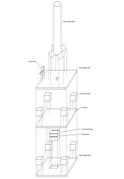
The high-level logical structure of the device is shown below:
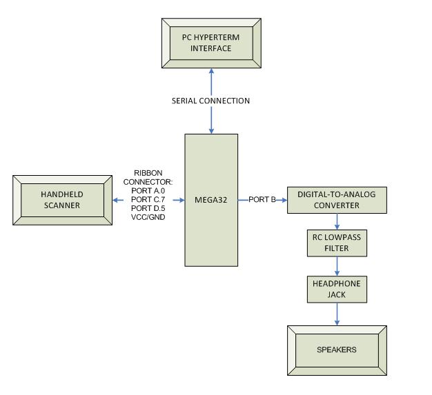
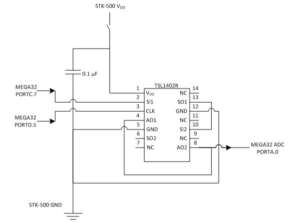
To summarize the block diagram: The Mega32 connects with the PC Hyperterminal interface at initialization, and the user inputs the desired clef and key signature. Then, the Mega32 begins reading and processing data from the handheld scanner through the Mega32 ADC (Port A.0), while the image sensor is controlled by interrupt-driven timing pulses from the Mega32 (from Ports C.7 and D.5). When the image processing algorithm and note recognition state machines running on the Mega32 determine that a note should be played, the DDS algorithm runs to ouptput a signal to the external digital-to-analog converter (DAC) attached to Port B. The output of the DAC is lowpass filtered to eliminate high-frequency buzz, then sent through a standard headphone jack to a set of computer speakers. The details of these steps are described in later sections.
Hardware / Software Tradeoffs
Even though we were limited by the performance of the microprocessor, we decided to use an image sensor with unprocessed output combined with more sophisticated processing algorithms to minimize cost. Furthermore, we were constrained by our lack of knowledge of optics and our inability to have precise positioning of the sensor. We were thus unable to take full advantage of the high sensor resolution. A third tradeoff was the use of backlighting to illuminate the area under the scanner (instead of projected light, as in an optical mouse). The combined effect of these constraints was that the image processed by the microcontroller was usable, but not optimal.
Compliance with Standards
Since the image sensor operats by a unique communications scheme, and we did not use any radio communication, there are not many standards applicable to our project. The only relevant standards are the RS-232 serial communication standard used to communicate with hyperterminal on the PC and the ANSI C standards.
Hardware Design
Back to Top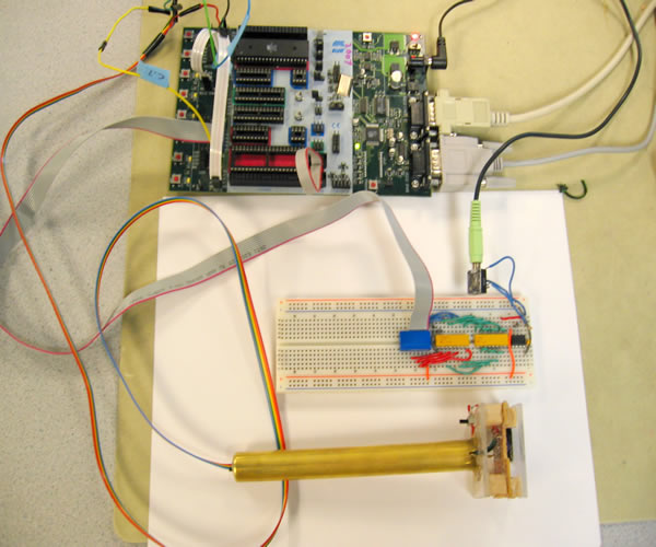
Scanning Wand
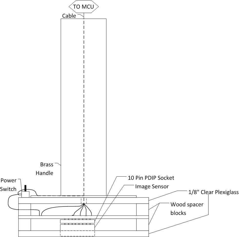
The design of the handheld scanning wand is simple, and serves only to provide a stable platform for moving the image sensor across the page. A six-inch piece of 5/8 inch diameter brass tubing serves as a handle, with a plastic cap sealing the tube on the upper end. On the lower end of the handle, the tube is slotted on its four cardinal points and splayed out to form "feet", which are attached to a 2" x 2" square of 1/8" clear plexiglass using hot glue. On the other side of the plexiglass are four small wooden spacer blocks roughly 3/8" thick in each of the four corners, similarly attached using hot glue. A DIP solderboard is hot-glued to the bottom of these. The DIP solderboard, cut to a 2" x 2" square, contains the wired image sensor circuit (schematic available in the Appendix). The DIP socket and image sensor are placed on the bottom side of the DIP solderboard, facing downward. Attached to the bottom of the solderboard are four more wooden spacers, to which a second 2" x 2" sheet of plexiglass is attached to protect the image sensor. These blocks are measured so that the bottom surface of the plexiglass is roughly level with the active surface of the image sensor, which sits in a cutout cut in the bottom plexiglass sheet.
During testing, it became clear that unwanted light was being projected onto the image sensor through the sides of the apparatus. To prevent this from happening, we wrapped a single turn of very narrow electrical tape around the lip of the active surface of the image sensor. This shields the sensor from all light except light coming directly through the page.
The plastic cap at the top of the brass tube as well as the top sheet of plexiglass at the bottom of the glass tube have small cutouts to allow wires to run from the solderboard to the STK500 via a ribbon cable. We placed a power switch in series with the Vcc line in order to protect the image sensor during testing. All other wires ran directly from the STK500 board to the solderboard on the handheld scanner.
An expanded diagram of the handheld scanner construction can be found in the Appendix.
Image Sensor
We sampled the TSL1402R linear image sensor from Texas Advanced Optoelectric Solutions. The image sensor we choose is a 256x1 pixel linear array made up of a line of 256 photodiodes. It has a 400 DPI resolution, with each pixel measuring 63.5 micrometers by 55.5 micrometers with an 8 micrometer spacing between pixels. It requires a 5V power supply, a ground supply, and a clock at any speed between 5KHz and 8MHz. The photodiode data is integrated (by an opamp-capacitor integrator), and output as an analog value between 0 (black) and 255 (saturated white). The pixels are output sequentially on each clock cycle after a start pulse (SI pulse). Thus, the output of the array is a series of analog values which represent each pixel value.
In addition to starting the output of the pixel data, the SI pulse serves another function. SI stands for "start integration". The entire time between the SI pulse on one cycle and the SI pulse on the next cycle, the photodiode data is being integrated. The data that comes out during any pixel line is the data that was integrated during the output of the last line. The longer the integration time is, the more easily the sensor is saturated by light, the shorter it is, the less sensitive it is. Since the SI pulse cannot be received until after the entire line of pixels is output, the minimum integration time is the length of time it takes to output a line of pixels. This is controlled by the clock speed, so ultimately the clock speed controls the integration time, and thus the sensitivity of the sensor.
We wanted a sensitivity that gave us good distinction between the black and white on the page, but did not saturate the sensor due to ambient light. Another factor to consider was that the internal ADC, which we used to read the pixel values, can only run as fast as 15KHz. This means that when the pixels are being read, we cannot run the output clock faster than 15KHz. After extensive testing, we determined that there was no single clock rate that was both slow enough to run the ADC and fast enough that the pixels were not saturated by ambient light. This forced us to run the clock at two rates. The clock rate alternates between running quickly for at least one full pixel line to set the integration time, during which the pixel data is not read, and then running much more slowly for one pixel line as the pixel data is read out. Thus, the integration time can be kept low while the data can be read at a reasonable rate.
Lighting the Image Sensor:
We needed a light source that was diffuse enough that it lit the page evenly so different pixels would not see different light levels. At the same time, the light had to be focused on the page and not shine any light on the sensor itself, or the sensor would saturate. This was inordinately difficult to acheive with the resources we had, so we decided to backlight the music instead of lighting from the top. This had the advantage that there was diffuse, even light across the page, but there was also no light shining directly on the sensor. Black markings on the page blocked the light more than the white spaces, making them distinguishable in the pixel output.Optics:
Ideally, we want the image sensor to be focused exactly on the music. However, due to our extremely limited knowledge of optics, we did not know what to expect when we put the sensor down on the music. Unfortunately, what we found is that the data was blurry due to focusing problems. We found the width of the spaces between staff lines to appear the same as the width of the lines themselves, which is not accurate. This made the image processing very difficult to make completely accurate.DAC
We based the design of the R/2R DAC on the diagram provided by Professor Bruce Land on the ECE 4760 website. A schematic of the DAC can be found in the Appendix. We used the 10k and 20k PDIP resistor packs in the lab to ensure that all of the resistors were well matched. Unfortunately, these packs each have 8 resistors, meaning the full circuit would require an extra resistor in addition to the packs (since 8 is exactly the number of pins we need to convert). This is not ideal, since it would be difficult to find a resistor matched to the resistors in the packs. At Professor Land's suggestion, we dropped the lowest ordered bit in the DAC, and used only the PDIP resistor packs for the whole design. This did not affect the accuracy much, as the lowest bit is within the error range of the DAC anyway.
To match the load impedance (very small) to the impedance of the DAC, we designed a unity gain buffer amplifier using an LM 358 op amp from the lab. Since the opamp saturates at 3.5 volts, we centered our output around 90, making sure that it never got above 150. To get rid of any high frequency noise we used a simple RC filter on the output with cutoff frequency 3.18KHz.
Software Design
Back to TopMain Program Loop
The code executes in the following order: First, all variables, ports, and control registers are initialized. Next, the user is prompted to enter the clef and key signature of the music in hyperterm. This data is stored in variables ksVal and clef_char so that when a note is played, the correct octave and sharp or flat of the note is played. Next, the music is scanned, and the data for one line of pixels is read into the imLine array. This line of pixels is then processed by the proc_image() method.
proc_image() updates the noteOn variable to reflect the location of a note if a note is found, or to reflect that no note was found. If a note is found, the value in noteOn can be a value between 0 and 10, 0 being the note in the space above the top staff line (G), and 10 being the note in the space below the bottom staff line (D). If a note was not found, noteOn is set to 11.
After the image is processed, there is a state machine in the main method that determines whether or not a note should be played; a state diagram for this state machine can be found in the Appendix. A note is only played if it is found in four of the last five samples. This is to reduce error in case there is any spurious data between note detection. The state machine has four states, start, foundNote, playNote, and maybeDone and maintains a 5 scan buffer called prevNote. The machine begins in start. If anything other than 11 (no note) is found in noteOn, the machine stores the noteOn in the buffer and moves to foundNote. After every scan between this point and when a note is played, the new note value is shifted into prevNote and then prevNote is checked for 4 repeats. If 4 repeats are found, then the machine moves to playNote and the note to be played is placed in noteToPlay. The playNote state maps the noteToPlay value to the actual note that needs to be played based on the clef and key signature from hyperterm. It uses two switch-case statements based on noteToPlay, clef_note, and ksVal and assigns the proper value to the note variable. This variable is used as a lookup table in the DDS increment table and determines the fundamental frequency that is played. At this point, the DDS is initialized, and the timer0 interrupt is turned on to begin the DDS. The state machine then moves to maybeDone. At this point, four out of the last five scans must contain no notes in order for the machine to move back to start.
Main takes care of one more important function, which is reset. If the user wishes to restart the program, maybe to reset the key signature or clef, he or she can simply type reset in hyperterm. This re-initializes all variables and restarts the hyperterm interface. The input from hyperterm is received by receive ready interrupt to minimize the impact of the receive on the rest of the program.
Image Sensor Control
All of the timing for the image sensor is controlled by timer 1. Timer 1 is set to toggle on compare match, and OCR1A changes betwen a low (fast) value and a higher (slow) value depending on whether an integrate cycle or a read cycle is running. The toggling output, which is the clock for the image sensor, comes out on pin D.5, and an interrupt is thrown at every compare match. The number of integrate lines between read lines is variable and defined by integrateCycles. The number of successive read lines is never more than 1. The value of the sensor clock signal is recorded at the beginning of every interrupt so that we can be sure whether we are on sending a clock high or low. To define a full line of pixels, the variable clockCounter counts the number of high sensor clock values (full periods of the sensor clock) up to 257. On the 257th cycle, a new SI pulse can be sent and a new line of pixel output can begin. The SI pulse is sent simply by setting pin C.7 high for 1.5 sensor clock periods, ensuring that at least one high clock edge coincides with the SI pulse. This happens regardless of whether we are integrating or reading, because a new line is always initiated when the previous line finishes. This entire method is prevented from running if the image processing algorithm is running (scanReady == 0) or if a note is playing (notePlaying == 1);
During integrate lines, no pixel data is read, so the code simply counts sensor clock periods until 257, sends an SI pulse, and restarts. During the read cycle, the pixels are read in by the ADC. The pixels are output from the sensor sequentially on each rising edge of the sensor clock. To give the output time to settle, the ADC is set to start a conversion on the falling edge of the sensor clock. This conversion is not read until the falling edge of the next sensor clock, where it is stored in an array of pixel data to be processed (imLine).
We chose to use 200 for the value of OCR1A during the integrate lines and 800 during the read line. Using 3 integration lines before reading, this gives a total time of around 45ms per read.
Image Processing
The image processing component of the software is by far the most complex. The image data is received from the image sensor in the form of a 256-element array containing integer values between 0 and 255. Analysis of a line of image data takes place in the following steps:
- Identification of Peaks and Troughs (Peak-Picking)
- Note Detection
- Dynamic Quantization
- Indentification of Absolute Staff Position
- Note Indentification
1. Identification of Peaks and Troughs
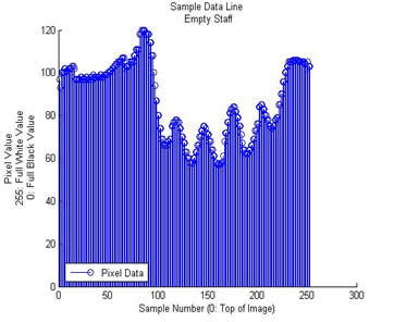
Our intial hope was to quantize each line of image data based on a previously determined constant value. However, analysis of acquired data shows that this is impossible. Due to the imperfect optics of the scanning wand, the nominal (white) light projected onto the sensor is not uniform along the length of the pixel array, and subsequently the features of the image scan appear to be multiplied by a concave envelope, as seen here:
 |
 |
The large troughs in the image data correspond to black features in the image (such as notes and staff lines). However, since the bottoms of these troughs are not at a uniform height, we cannot perform quantization with a single black/white threshold value. Instead, we need to run a dynamic quantization algorithm which compensates for the varying trough depths and peak heights. In order to accomplish this, we use a peak-picking algorithm to identify the positions of major troughs and peaks, then determine a quantization value for each individual trough.
For the purposes of the peak-picking algorithm, we make the following definitions:
We define the vector of pixel indices as
Y = [ 0 1 ... 254 255 ]
and the vector of pixel values as
A = f(Y) = [ f(0) f(1) ... f(254) f(255) ]
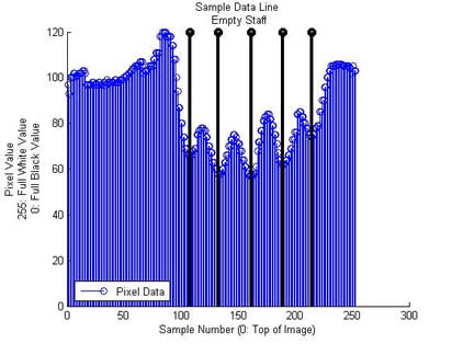
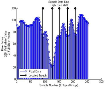
The peak-picking algorithm uses the first derivative df/dY of the data line to identify the local minima and maxima along the contour. To smooth the curve to avoid detection of spurious features, the derivative is evaluated by calculating the amplitude difference between every fourth point. As df/dY is evaluated along the contour, troughs are detected by detecting a change in the sign of the derivative. For the five troughs in the contour with the lowest trough values f(y1), f(y2), ... , f(y5), the values f(yn) and yn are sorted in ascending order of yn and stored in the array troughs. Once the troughs have been identified, we iterate through the portions of the image line between the troughs to find the local maxima. The amplitudes of these four maxima and their indices are stored in the array peaks. The results of the peak-picking algorithm after execution on the previously plotted data are shown here:
 |
 |
2. Note Detection
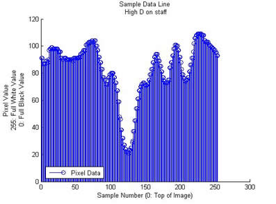
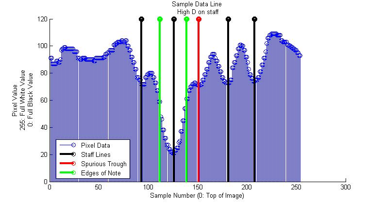
Our analysis of the data revealed that the peak-picking algorithm detects three kinds of troughs: staff line troughs, note troughs, and spurious troughs. All of these can be observed on the sample image data shown above. Once the locations and magnitudes of the troughs and peaks have been measured, we analyze each trough and the peaks on either side of it to determine whether it is a note trough. First, we search for a trough with height less than the average of the four other trough heights. This trough is flagged by setting notePresentFlag equal to its location in the troughs array. Second, we check to see if the height of the flagged trough differs from the average of the four other trough heights by at least some value deltaH. If the difference is less than deltaH, the flagged trough is deflagged, since it is most likely either a spurious trough or a staff line trough with slightly abnormal depth. In the previously plotted data, there is no effect on the "empty staff" dataset since notePresentFlag is not set after note detection. The values set for the "High D on staff" dataset are shown below. Note that one of the troughs is flagged as "spurious"; a trough is tagged as "spurious" at a point later in the algorithm, but the information necessary to detect a spurious trough has all been gathered at this point. Any troughs which are not notes and are not spurious are assumed to be staff lines.
We can assume that any exceptionally deep and wide trough is a note by considering the optics of the scanner wand. Since the image is not completely in focus, it is reasonable to assume that a thin black feature (such as a staff line) would allow more light to pass around it and strike the sensor than a thicker black feature (such as a notehead). Thus, we would expect that a note trough would be much deeper and wider than a staff line or spurious trough.
3. Dynamic Quantization
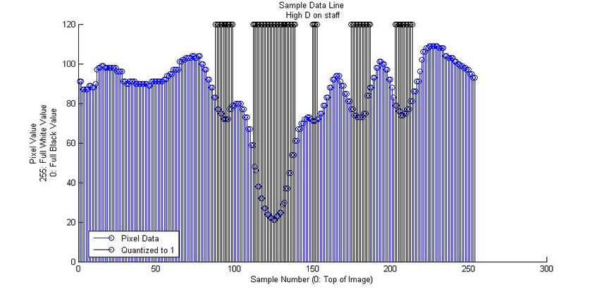
Assuming that a note trough has been identified (the method exits if notePresentFlag = -1, the unflagged value), the next step in the algorithm is to determine the widths of the sections of the image lines which are seen as "black" by the sensor. We determine the width by first determining some value Qval, and then setting pixels with value greater than Qval equal to 0 and pixels with value less than or equal to Qval equal to 1 (quantization). This is necessary to determine the the locations of the top and/or bottom staff lines in the next stage of the algorithm.
Since the trough minima have high variation (both between individual troughs and between images), we cannot use a single Qval to quantize all the troughs. Instead, a Qval must be determined for each trough. For the trough n, we define Qvaln as
Qvaln = troughnvalue + 0.5(average(neighboring peak values))
The effect of the individual quantization of each trough is to effectively normalize the bottom of each trough to zero, thereby eliminating the concave envelope effect observed in the original data. The indices of the beginning and end of each chunk of 1's are stored in chunkStartN and chunkEndN, where N is the trough number. Since the ranges assigned for the dynamic quantization are determined based on the positions of troughs and their neighboring peaks, these assignments are error checked to avoid overflow problems when computing index values. The result of quantization for the "High D on staff" data is shown below.
4. Indentification of Absolute Staff Position
With the quantization complete, we can examine the data extracted from the image to determine the absolute position of the staff. At this point in the image processing, we have obtained:
- Locations and amplitudes of the five deepest troughs in the image line
- Locations and amplitudes of the four peaks between the five deepest troughs
- Widths of the five deepest troughs
- Flag on a trough which contains a note (by virtue of being exceptionally deep and wide)
We can now make a decision on whether or note a particular non-note trough is "spurious". We define a trough as spurious if:
- The width of the trough is 20 or less
- The width of the trough is greater than 50
- The minimum value of the trough is greater than 105
- The trough has not been flagged by notePresentFlag
where the constant values used in these decisions were obtained through repeated trial and error. Given this information, the absolute positioning of either the bottom or the top staff line is obtained using the following logical tree:
        if (first line not very thin)
              if (first line is flagged as the note)
                    FIRST LINE IS A NOTE
                    SKIP TO END AND START FROM THERE GOING BACKWARDS
              else
                    FIRST LINE IS TOP STAFF LINE
                    USE RELATIVE POSITIONING FROM THERE
        else
            FIRST LINE IS SPURIOUS
            GO TO NEXT LINE AND RESTART TREE
Once the absolute position of either the top or bottom staff line has been identified, we are ready to identify the note based on its relative position within the staff.
5. Note Identification
We confined our problem to notes which are placed on the staff, leaving us with the following set of eleven possible notehead placements:
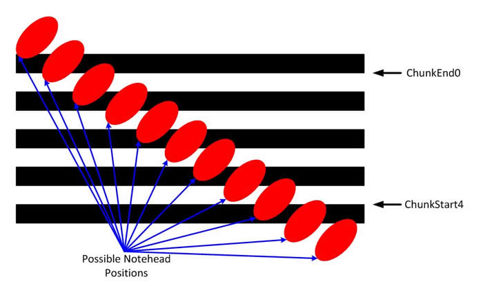
Furthermore, we know that either chunkStart4 contains the index of the top of the bottom staff line or chunkEnd0 contains the index of the bottom of the top staff line. Assuming that the center of a note trough corresponds to the center of a notehead on the staff (an assumption which was confirmed by examining a large number of data sets), we can identify the note by calculating its distance from the known staff position (in terms of the width of staff lines and spaces). This process is streamlined by calculating and storing a number of additive coefficients during initialization; this reduces the number of additions required during the process of determining the location of the notehead. The location of the notehead is assigned as a number from 0 to 10 (with 0 corresponding to the top of the staff and 10 corresponding to the bottom) and placed in the variable noteOn. This marks the completion of the image processing algorithm.
Vulnerabilities of this Image Processing Algorithm
We have been able to identify several cases which cause this image algorithm to detect a wrong note or fail to detect a note. All of these involve either the criteria for spurious troughs or the addition / subtraction used for the relative positioning of the note trough on the staff. The reason that these two components of the algorithm are vulnerable is that they are not dynamic in any way, and thus are subject to failure when conditions vary during use. Since we make decisions based on predefined (experimentally determined) values, we run the risk of making errors on data which is abnormal in some way. Although analysis of our data shows that these faults are the cause of nearly all errors in note-reading, we determined that both computational and labor-time constraints would make implementation of dynamic components too difficult.
Hyperterm Interface
Hyperterminal is used in our project to implement a simple user interface so that the user can set the clef and key signature of the music to be scanned. Once these values are set, the correct notes will be played according to the those settings. In addition, hyperterm is used to reset the program to re-initialize all variables and restart the clef and key signature prompt, in case the user would like to change those settings. The code is fairly simple to understand, and is contained in promptUser() and read_terminal(). The microcontroller prompts the user to input a clef, either 'B', or 'T'.
The microcontroller then begins scanning the input to hyperterm using read_terminal(). This is implemented by a while loop that runs until the user hits enter. In the while loop, the receive ready flag is continuously polled until it is high. Then the character is recorded using getchar() and echoed using putchar. If the char is not a backspace and not an enter, the char is added to a buffer and the while loop is run again. If the character is a backspace, a small backspace code deletes the last character entered from the buffer, prints a space and then a backspace to hyperterm to clear the last character entered, and then reexecutes the while loop. Finally, if the char entered is an enter, the method returns to promptUser(). promptUser() checks the input to make sure it is a 'B' or a 'T'. If it is not 'B' or 'T', the user is prompted again, and a new read_terminal() is initiated. If the input was 'B' or 'T' the appropriate word 'bass' or 'treble' is saved in variable clef for printing later in this method, and the 'B' or 'T' is saved in variable clef_char for note octave determining when a note is played. This process is repeated for the key signature. The name of the key signature is stored in ks for printing at the end of the method, and a number corresponding to the key signature is stored in ksVal for note sharp/flat determining when a note is played.
The receive for the reset signal is slightly different. For the initial interface, it did not matter if the receive was continuously polling or looping because there was nothing else running. Since the reset receive runs continuously in the background while all of the scanning is occuring, it is interrupt driven. It uses the receive ready interrupt, so it only uses getchar() when a char is input to hyperterm. The buffer is built the same way as before, and the input is checked in main after the user hits enter. If the user typed 'reset', then the code is reset. All variables are reinitialized and the hyperterm interface prompts the user for a clef and key signature again.
DDS
The scheme described for DDS in the "Background Mathematics" section is implemented in software without any noteworthy changes from the description above.
Results
Back to TopOur project ran at around 38ms per scan, plus probably one or two milliseconds for the image processing algorithm. This time means that the user has to move the wand fairly slowly to ensure enough samples on each note to identify and play the note. This speed was limited mostly by the ADC. If we had used an external ADC, we could have cut this time down significantly, probably to around 12-13ms, which would have made scanning much easier for the user.
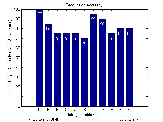
The accuracy of the scanner is not perfect. Below we have a histogram of the percentage of correct note identifications out of twenty trials for each note. Each trial consisted of starting the image sensor off the paper, placing it on the note, and recording whether the correct note was played. Overall, the error rate is around 74%. We spend a long time improving this error rate by tweaking the image processing algorithm. The algorithm that we have written is about as good at recognizing the notes as we think it can be, given the blurred data from the image sensor. Given the raw data, we don't think a human would do better at identifying the notes than the algorithm.
Furthermore, due to the poor image quality and the computational limits of the microcontroller, we were forced to limit the kinds of scannable music to a relatively small subset of musical notation. Currently, the device is programmed to recognize only quarter notes on a clear staff. The image processing algorithm will produce erroneous results if any of the following are encountered during scanning:
- Accidentals (sharp, flat, or natural signs mid-staff)
- Chords (multiple notes stacked on top of each other)
- Any note type other than quarter notes or eigth/sixteenth/32nd notes with small flags (no bars)
- Ties between notes
- Repeats or any other kind of thick bar lines
- Rests of any kind
- Key changes
- Accents or other dynamic markings
The accuracy of the music synthesis is nearly perfect. The notes that are played match the notes that are identified by the wand, even though they aren't always the same as the note written on the page. Since the DDS is so complex, it is difficult to measure the actual frequency being played. Thus, at professor Land's suggestion, the note accuracy was verified by a group member comparing the notes to the notes as played by a computer program.
There are no real safety concerns regarding our project, other than possibly hurting one's ears due to high music volume or hurting one's eyes due to looking directly into the overhead projector.
Our project has little chance of producing electromagnetic interference, because it does not transmit on any frequency. The one slight interference issue is due to random noise produced by the overhead projector, which was large enough to be noticeable on a digital multimeter measuring AC voltage. However, groups that were using RF communication did not seem to notice a noise difference when the projector was on.
The project is very useable by anyone with a steady hand. It is intuitive and does not involve a lot of input from the user. As long as the user scans the music slowly and does not overly rotate the wand, anyone can play music with our wand.
The accuracy of the image algorithm for the possible note positions is shown here:
Conclusions
Back to TopWhen we first envisioned the idea of an optical music-scanning sensor, we knew that the problems of image processing on the microcontroller would be difficult to solve. Furthermore, we knew that we would have to make some sacrifices with regards to the optics of the system, considering our lack of knowledge of optics and our somewhat imprecise construction. With this in mind, we set out to see if we could build a system that would perform optical note recognition and synthesis to a reasonable degree of accuracy, and we are pleased that we have achieved the current level of performance.
It is easy to see room for future improvements. The major opportunity for improvement is the construction of a system which takes advantage of the high optical resolution of the image sensor to obtain better image data, which can be analyzed with a higher degree of accuracy. Furthermore, with a high-resolution image, it become possible to recognize a wider set of musical notation (different types of notes, accidentals, etc) by performing symbol identification with correlation. A significantly improved version of our device might be one with improved optical resolution and a more powerful processor which is capable of carrying out a more complex image processing algorithm involving multiple correlations.
A second area for improvement is consolidation. With some enlargement and modification of the structure of the handheld wand, the microcontroller, a battery, the DAC, and a small speaker could be placed in or around the handle of the wand, making the device completely handheld and wireless. The functionality of the PC hyperterm interface could easily be replaced with a small LCD screen and a series of buttons without sacrificing convenience. The most difficult part of making a wireless version of the device would most likely be building an attachment to the scanning end of the device to project light onto the scanning surface (like an optical mouse), instead of backlighting the music to be read.
No code was taken from the public domain, and our project does not involve reverse-engineering some design. There are no legal considerations relevant to our project. We have considered the idea of patenting the concept of a real-time embedded optical music scanner, but have not yet come to a decision regarding a course of action.
Ethical Considerations
As students in the Cornell University School of Electrical and Computer Engineering, we acknowledge the IEEE Code of Ethics and state that its principles were followed closely during all stages of design and development of our project. We maintain that the Music Wand may be used by any member of the public without endangerment of health or safety, and note that all actions taken by our team during development were carried out with neither false nor malicious intent. In any instance where our actions had the potential to cause a conflict of interest or harmful effect, we searched for any and all possible alternatives and endeavored to choose a course of action which eliminated any negative effect on us and all others. We contend that the sole purpose of our project was the advancement of our technical competence and understanding, and that no design decision was made without consideration of its potential consequences. No monetary or other incentives were provided during development of our project, other than the usual criteria of academia. We acknowledge that our design contains flaws, some of which we have noted and others which remain undetected. We have reported all known data and honestly and realistically evaluated our own work, and we welcome any and all constructive criticism from both our teachers and our peers. Furthermore, we welcome the opportunity for additional discussion on topics relevant to our work, both with and without in regards to our own project. Finally, we note that any and all contributions to our work from other parties are fully credited, and we extend our thanks to all contributors.
Acknowledgements
We would like to extend our thanks to Adam Hart, Morgan Jones, and Donna Wu for the use of their DDS scheme and code (see Guitar Synthesizer), and to Texas Advanced Optoelectronic Solutions for their donation of the image sensor used in the device. Above all, we thank Bruce Land and the ECE476 staff for providing both materials and invaluable advice during the development of our device.
Appendix
Back to TopTasks
Nick Hoerter conducted the background research for the DDS portion of the project, and wrote the code which implemented the DDS algorithm, and decided on the design of the resistor ladder DAC. Nick also implemented the timing and control for reading data from the image sensor. Tom Chatt was responsible for the design and writing of the image processing algorithm, and both members worked on the development of the Hyperterm interface, hardware construction, general background research, and writeup.
Component List and Costs
| Quantity | Item | Unit Price | Total Price | Notes |
| 2 | 2 Pin Jumper | $1.00 | $2.00 | Lab Rental |
| 1 | 10 Pin Jumper | - |
- |
Lab Materials |
| 1 | 6 Pin Jumper | - |
- |
Lab Materials |
| 3 | 1 Pin Jumper | - |
- |
Lab Materials |
| 1 | 14 Pin PDIP Socket | $0.50 | $0.50 | Lab Rental |
| 1 | White Board | $6.00 | $6.00 | Lab Rental |
| 1 | 6" DIP Solder Board | $2.50 | $2.50 | Lab Materials |
| 1 | 1/8" Clear Plexiglass sheet | - |
- |
Donated by Bruce Land |
| 1 | 5/8" Brass Tubing | $3.69 | $3.69 | Cornell Store |
| 1 | 3/8" Wood Spacer | $1.19 | $1.19 | Cornell Store |
| 1 | Plastic Cap | - |
- |
Scrap Material |
| 2 | PDIP 8 Resistor Packs | - |
- |
Lab Materials |
| 1 | LM358 Op-amp | - |
- |
Lab Materials |
| 2 | 0.1 microFarad capacitor | - |
- |
Lab Materials |
| 2 | 1K Resistor |
- |
- |
Lab Materials |
| 1 | Headphone Jack | - |
- |
Lab Materials |
| 1 | Mechanical Switch | - |
- |
Lab Materials |
| 20 | Sheets of printer paper | - |
- |
Lab Materials |
| 1 | TAOS TSL1402R Image Sensor | - |
- |
Sampled from TAOS |
| 1 | Overhead Projector | - |
- |
Phillips Hall (borrowed) |
| 1 | Set of Computer Speakers | $5.00 | $5.00 | Lab Rental |
| 1 | Desktop PC | - |
- |
Lab Materials |
| 1 | STK500 | $15.00 | $15.00 | Lab Rental |
| 1 | Power Supply | $5.00 | $5.00 | Lab Rental |
| 1 | Atmel Mega32 | $8.00 | $8.00 | Lab Rental |
| Total Cost | $43.88 |
Schematics
Digital-to-Analog Converter (DAC) Circuit
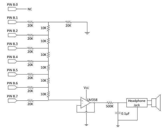
Image Sensor Circuit
Expanded Diagram of Scanner Construction
Other Appendices
TAOS TSL1402R Linear Image Sensor Datasheet
Information on key signatures and musical notation
DDS Increment Values:
| Note | Freq. | Inc. | Note | Freq. | Inc. | |
| C2 | 65.406 | 4494666.093 | C4 | 261.63 | 17979077 | |
| 69.296 | 4761984.857 | 277.18 | 19047665 | |||
| D2 | 73.416 | 5045109.101 | D4 | 293.66 | 20180162 | |
| 77.782 | 5345138.337 | 311.13 | 21380691 | |||
| E2 | 82.407 | 5662965.916 | E4 | 329.63 | 22652001 | |
| F2 | 87.307 | 5999691.352 | F4 | 349.23 | 23998903 | |
| 92.499 | 6356482.875 | 369.99 | 25425519 | |||
| G2 | 97.999 | 6734439.997 | G4 | 392 | 26938035 | |
| 103.83 | 7135143.266 | 415.3 | 28539199 | |||
| A2 | 110 | 7559142.437 | A4 | 440 | 30236570 | |
| 116.54 | 8008567.815 | 466.16 | 32034271 | |||
| B2 | 123.47 | 8484793.788 | B4 | 493.88 | 33939175 | |
| C3 | 130.81 | 8989194.747 | C5 | 523.25 | 35957466 | |
| 138.59 | 9523832.276 | 554.37 | 38096016 | |||
| D3 | 146.83 | 10090080.76 | D5 | 587.33 | 40361010 | |
| 155.56 | 10690001.8 | 622.25 | 42760694 | |||
| E3 | 164.81 | 11325656.95 | E5 | 659.26 | 45304002 | |
| F3 | 174.61 | 11999107.83 | F5 | 698.46 | 47997806 | |
| 185 | 12713103.19 | 739.99 | 50851726 | |||
| G3 | 196 | 13469017.43 | G5 | 783.99 | 53875383 | |
| 207.65 | 14269599.34 | 830.61 | 57079085 | |||
| A3 | 220 | 15118284.87 | A5 | 880 | 60473139 | |
| 233.08 | 16017135.63 | 932.33 | 64069230 | |||
| B3 | 246.94 | 16969587.58 | B5 | 987.77 | 67879037 | |
| C6 | 1046.5 | 71914932 |