|
Harnessing the power of Doppler Radar to show you the power of Mother Nature, the Weather Canvas is a wireless weather monitoring system that makes the boring task of getting the days weather a more colorful and vibrant experience.
Introduction
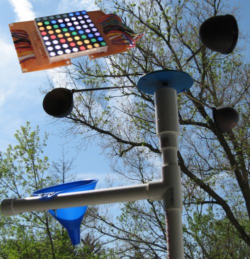
The Weather Canvas is a robust outdoor weather monitoring system coupled with an indoor LED display. The outdoor system consists of a microcontroller, temperature sensor, humidity sensor, home-made anemometer, a Hot Wheels radar gun modified to measure precipitation, and a solar panel to measure sunlight and charge the microcontrollers power source. Once per minute, the system transmits the data it has collected to the indoor microcontroller by a 433 MHz RF signal, where the signal is decoded and the information is displayed as a sequence of five vibrant images on the 8x8 RGB LED matrix. The images chosen by the system depend of the weather conditions transmitted. The indoor system uses pulse width modulation (PWM) to provide millions of potential colors to each pixel, allowing for limitless image possibilities.
High Level Design
Rationale
This project was a combination of several core components we wanted to include. Radio frequency communication seemed like an interesting concept to implement, and we were trying to figure out ways to integrate the Hot Wheels radar gun for a long time. Its ability to detect motion was appealing, and we considered doing an invisible fence that is not painful to pets. The Weather Canvas idea came from browsing the Spark Fun website, where we saw an 8x8 RGB LED matrix, and we wanted our project to use it after watching some YouTube videos. Our shared interest in renewable energy led us to solar power, and these ingredients came together for the perfect recipe: a weather monitoring system. After we had decided on the concept, all of the pieces started falling into place: RF to communicate with an indoor unit using the RGB LED display, radar to measure rainfall, and solar power to measure and harness sunlight. The temperature, humidity, and wind sensors followed naturally. We knew integrating these several separate parts would be a challenge but were willing to undertake it to see the final result.
Logical Structure
The most important feature of this project is the RF communication between the outdoor and indoor unit. Without it, the LED matrix would have nothing to display and the outdoor monitoring unit would keep the information for itself. The data path starts at the sensors, whose information is collected by the outdoor MCU. It relays this information indoors with the RF encoder/transmitter. The receiver/decoder unpacks the data for the indoor MCU, which then determines the images to display on the LED matrix based on the data it is has received.
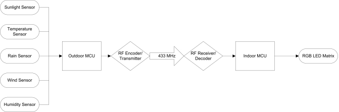
Figure 1
Hardware/Software Tradeoffs
Early in our project design, we had to decide how to implement RF. Our first instinct was to replicate the system used by Meghan Desai in her Wireless Telemetry project. We had allotted the price of the RCT-433 transmitter and RCR-433 receiver and were preparing to write all the encoding/decoding code, which appeared intimidating. Bruce Land made a comment as an addendum to his talk about RF regarding an integrated circuit by Holtek which encapsulates the encoding and transmitting protocols into one hardware unit. After being redirected by several companies including Digikey, we found a supplier at Rentron who was eager to sample us the Linx Technologies RXD-433-KH2 receiver/decoder and TXD-433-KH2 transmitter/encoder modules. The units eliminated the need for software encoding or decoding protocols, solving a software problem in hardware. The fact that they were free made our decision even clearer. One can simply drive the data line with the data to be transmitted, the address line with a unique address (which can be a series of hardcoded ones, zeros or floating) and assert the TE (transmission enable) pin. Any receiver with its address pins configured the same way will have its VT (valid transmission) pin go high and its output data line mirror that of the transmitter.
Indoor Display Unit
Hardware Design
The LED Canvas is an 8x8 LED matrix, where each pixel actually consists of 3 discrete LEDs: one red, one green and one blue. It is connected to a prototype board fitted with a regulator to allow the microcontroller to power from a wall socket, so no batteries are required. Figure 2 shows the pin configuration of the LED matrix. The black square shows the location of each pixel. The pixels require 4 pins for control: the three color controls, shown by pins 2, 1, and 32 in Figure 2 for the first pixel, and a base pin (or row pin), which is grounded when the pixel is on. Each pixel can simply be made to take on 8 different colors by asserting ones and zeros across the pins of each LED. For example, the first pixel can be made purple by asserting ones on pins 1 (red) and 2 (blue), and zeros on pins 32 (green) and 26.
As is evident from Figure 2, controlling each pixel individually becomes an interesting task since each column of pixels shares the same color control pins (2, 1, and 32 are color control pins, with pin 2 controlling the blue LEDs in the first column, etc ), with only the base pin to differentiate pixels in a column. The way around this control issue is to cycle through the rows, asserting the control pins appropriately based on the desired color value of the pixel in the given row. Hopefully, this can be done quickly enough so that the viewer does not notice flickering. In the case of the Atmel Mega644 microcontroller used in this project, the 16 MHz crystal clock was indeed fast enough.
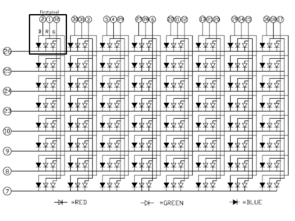
Figure 2
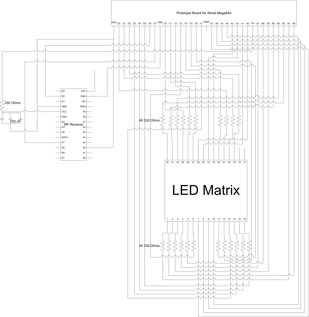
As can be seen from Figure 2 and the schematic in Appendix B, fully controlling the LED matrix requires 32 pins, the full pin complement of the Atmel Mega644 used for this project. Each color control pin must also have a corresponding current-limiting resistor (for a total of 24), as seen in the schematic. Table 1 shows the original pin mapping from the matrix to the Mega644 microcontroller. Unfortunately, two pins of the Mega644 were required for receiving RF signals relaying weather data from the outdoor unit. Pins D.6 and D.7 were chosen for this task, since they represent the red and green color control pins for the last column, localizing the damage. This left only 30 pins to control the matrix. An interesting solution to this problem was an increased length RF data transmission, which in addition to conveying the binary conditions outside (sunny/not sunny, raining/not raining, hot/cold, etc ), would display the severity of the condition using the available blue pixels of the last column. The severity meter will be discussed at length in the software section.
Table 1
The pin-out of the Linx Technologies 433 MHz RF receiver is shown below in Figure 3. It is not necessary to delve into the meaning of each pin since only a select few are necessary. ANT refers to the antenna, made from 16.5 cm of standard wire, sufficient for our purposes. GND refers to the microcontroller ground and likewise VCC refers to the microcontroller Vcc. VT refers to the valid transmission bit, which will be asserted if the decoder/receiver hardware determines that a valid transmission is being received. The value of VT is determined by the A0-A9 bits, which refer to the address. These pins must be synchronized between the transmitter and the receiver in order for a signal to be received. Finally, D0 through D9 refer to the data bits received during the transmission. If a valid transmission is received, these pins will mirror the data bits asserted on the receiver. To minimize the number of pins needed on the receiving side (so as to not cripple the LED matrix), only D0 is used. That is, the transmitter conveys all the necessary information bit by bit on D0, and the receiving side decodes and stores these bits (in software) until the full transmission is received. As seen in schematic Figure 2, the VT pin is connected to the microcontrollers D.7 port and D0 is connected to D.6. The address bits are hardcoded with a combination of floating and ground values. Also necessary on the RF receiver was a voltage dropping resistor to bring the voltage down since the maximum Vcc voltage of the receiver is 3.6 V. As seen in Figure 2, a 330 Ohm resistor was used. Finally, a simple RC circuit is set between the microcontrollers Vcc and that of the RF input to filter out noise, as recommended by the manufacturer. They recommended a 10 Ohm resistor and a 10 micro Farad capacitor, which corresponds to 300 nano Farads when using the 330 Ohm resistor. A 300 nano Farad capacitor was not available, so three 100 nano Farad capacitors were set in parallel.
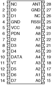
Figure 3
Software Design
In the Weather Canvas project, we did not want to be bound by the choice between only 8 colors. Utilizing the Pulse Width Modulation (PWM) technique, one can increase the available colors per pixel from 8 to a theoretical 16 million. The goal of PWM is to be able to modulate the amount of power received by a load, and in the case of the LED matrix, the amount of power received by each LED. This gives us accurate control over the color of the pixel. This technique is necessary since our digital microcontrollers are not easily capable of modifying the voltage they output, i.e. a digital one is Vcc, and Vcc is usually 5 Volts. To achieve this power modification, the following technique was used: a standard for-loop counts to a predetermined value, and during each iteration of the loop, values representing the fraction of time each color led should be on are decremented. When any of them reach zero, that particular led turns off. Once the for-loop reaches its maximum, the loop starts again on the next row. In this way, for each row, the leds on the row are on for a fraction of the total time, transferring varying amounts of power to each of them. To better understand, the program containing this method must be explained.
The augmentation of 32 pins many times per second as well as need to receive RF data required that thing happen in this program as quickly as possible, so that the user does not see the LEDs blinking on and off, which would degrade the visual experience. It is for this reason that the program contains no ISRs which may interrupt the program and only one function besides main. The general order of events is as follows: the program determines which picture in the five-picture sequence to display, determines the severity of the given weather condition portrayed in the picture, assigns colors to the pixels based on the picture it decided to display and the severity, then assigns PWM cycle values for each color control pin based on the current row. All LEDs in the row are turned on, and are then turned off at different points in the PWM loop, depending on the required intensity of the red, green, or blue LED for a given pixels color. This PWM loop is done once for each row. Next, the VT pin from the RF receiver is checked to see if a valid transmission is incoming, and if so that data is pushed into the buffer. Once the buffer becomes full, the data is parsed and transferred to the process which chooses the next picture.
The program, LEDPWM.c, is available to view in the Appendix. A series of #define statements near the beginning represent the color of a pixel given by its red, green, and blue hexadecimal values. E.G. for violet, red=3b, green=20, and blue=3b. These values used to be out of 255 (hex: FF), but for timing reasons to be discussed later, they had to be divided by 4, resulting in the possible creation of 262,144 colors (64*64*64) instead of 16 million (256*256*256). While this reduction is disappointing, it is still much better than 8 possible colors.
The shimmering() function is responsible for smooth picture transitions. The transitions between pictures are done such that all the LEDs brighten to white before changing the picture, so that when the brightness returns to normal, the next picture is being displayed without the user ever seeing the switch. This is done by steadily augmenting the PWM values of the pixels to gradually increase them to full brightness. Each time the shimmering() is called, it either increases or decreases the PWM values of the pixels by one unit up to a maximum augmentation of 100, so that after 100 cycles of the main loop (each with 256/4=64 iterations of the PWM loop), the LEDs are all white. The speed at which shimmering() reaches full brightness is augmentable via the counter variable, which when set will hold the shimmer factor constant for that number of cycles, thus slowing the brightening process. This was added since the transitions proved to be extremely fast, since the program runs through 100 loops in much less than one second. Once maximum brightness is reached, shimmering() then sets the switchpic value to 1, alerting the proper system to switch to the next picture, and makes the increment negative so that the LEDs will start darkening to normal levels, revealing the next picture in the sequence.
The main while loop starts by checking the switchpic variable to see if the shimmering() function has brightened the current picture enough to transition to the next picture in the sequence (the sequence is determined by picseq[], which is a size 5 array containing the picture values of the 5 pictures of current weather conditions to display, in order) and its corresponding strength (the strengths are contained in the size 5 array strength[], which contains values of either 0,1,3,5, or 8, depending on the severity of the weather condition of the corresponding picture). Then, depending on what picseq[] has assigned to be the current picture in the sequence (in the pic variable which holds the current picture ID) and what strength[] says is the current strength (in the currestrength variable), each pixel is assigned its color (using the #define statements above, so that each value in the size 64 pixel array contains the brightness for the red, green, and blue LED that control it). Table 2 below shows the picture indexes that are stored in the picseq[] array depending on what pictures are to be displayed. Figure 4 shows the possible displayable pictures. They were created in Excel and hard-coded into the program.
Table 2
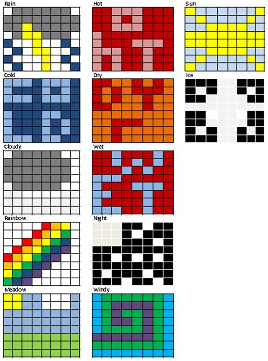
Figure 4
Next, a for-loop runs through each of the 8 rows (as was previously stated, color control pins are shared in the column, meaning the row is the only way to distinguish different colors), asserting one of the rows at a time. This means that at any given instant only one row is illuminated (by asserting the row to zero and the rest to one, letting current flow only in the grounded row, done by changing PORTA). For instance, if PORTA = 0b01111111, this means that row 8 is illuminated the rest are dark. Then, for each row (meaning for each iteration of this outer for-loop) the PWM values of each color control pin are set by parsing the value of the pixel variable for the red, green, and blue LED corresponding to each row. After the PWM values are set, all the LEDs are turned on and shimmering() is run to augment the PWM values if necessary (i.e. a transition is occurring). The variable hold determines how long each picture is displayed before transitioning to the next.
Finally, the PWM loop is initiated. At the beginning, all the LEDs are on, and throughout the iterations of the PWM loop, LEDs are turned off if their PWM value (which is being decremented with each iteration) falls below zero, thus transferring different amounts of power to each LED depending on how much of the period sees the LEDs on compared to off. The lower the initial PWM value, the shorter the duration of time the LED is on (and lower power transferred), and the dimmer it will appear as perceived by the human eye. Initially, the period of the PWM loop was 256, allowing the PWM value definitions to range from 0-255, which would have allowed us to use traditional RGB definitions to determine color. But after experimentation, visible flickering occurred, which hurt our eyes and could cause a possible safety concern. It was for this reason that the PWM period was experimentally reduced by a factor of 4, until there was no visible flickering. Before the current, successful version of the program was created, there were several failed attempts including the possibility of using hardware PWM to control the LEDs. This idea was quickly abandoned as 192 channels are required to control all the LEDs (64 pixels * 3 leds/pixel) and the Mega644 does not provide enough.
After the PWM cycle of each row, a simple check is performed on PIN D.7, which corresponds to VT of the receiver. If a valid transmission is being received and it is not the same data seen in previous cycles (thus the check of VTprev to make sure that new data is being received), the data is stored in the buffer. When the buffer becomes full (its size becomes 10 bits), the data is transferred to a temporary variable called nextset (freeing the buffer to become empty and receive more data), the buffer size is reset, and the index of picseq[] becomes zero so that on the next iteration of the main while loop, the new pictures will be displayed. After this is done, the temporary variable must be parsed so that the proper picture IDs are stored in picseq[] in the proper sequence, as well as the strengths of those weather conditions. The top of Table 3 shows the bit divisions of the 10 bit code according to weather condition and the rest of Table 3 shows the codex used to parse the data into the proper pictures and strengths. This ends the iteration of the main while loop and upon the next, as previously examined, the next (or first if new data was received) picture in the sequence will be displayed if appropriate (meaning if the pixels have all whited out in preparation for the transition).
Table 3
Outdoor Weather Station
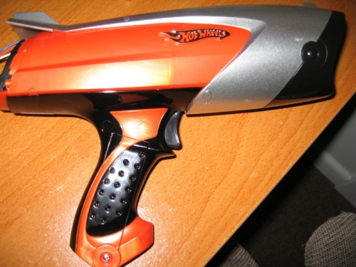
The outdoor weather station consists of five self-contained sensing units: temperature, humidity, solar, wind, and rain. All of the sensors except humidity ultimately output a voltage, which is fed into the multiplexed inputs of the ATmega644s analog-to-digital converter. The temperature sensor is an LM34 whose 10mV/degree F is fed into ADC7. A Honeywell HCH-1000-001 capacitive humidity sensor measures the moisture content of the air, outputting a varying capacitance rather than voltage. This required a repetition of Lab 1 (capacitance measurement), with adjustments to measure picofarads rather than nanofarads. A pair of Sun Power PWR1241 photovoltaic cells serve a dual purpose: to measure the intensity of sunlight and to recharge four NiMH AA batteries, allowing the outdoor unit to run for extended periods without battery replacement. The wind gauge is a homemade anemometer based on popular Easter Egg designs. It was made from scavenged parts, and at its core is a small DC motor that is spun by the Dinosaur Egg rotors and generates a voltage up to about 25mV. Finally, the most innovative element of the outdoor weather station is the Doppler Radar Rain Gauge, which is a modified Hot Wheels Radar Gun pointed skyward to sense the presence of falling rain. It was by far the most difficult part of the outdoor station, and this section begins with a description of its design.
Hot Wheels Doppler Radar Rain Gauge
The Hot Wheels Radar Gun is the most inexpensive functioning radar gun on the market, using Doppler Radar at a 10.525GHz operating velocity. It is designed for kids to measure toy cars and bike riders, but it provides an accurate measurement of velocity that has countless applications. For our purposes, it is sensitive enough to measure the velocity of falling rain and categorize it according to how far it has fallen. This project was originally proposed with a tipping bucket rain gauge that filled a receptacle at the end of a lever and indicated rainfall by tipping frequency. We were hesitant of this design due to its mechanical complexity and were looking for another method. By inadvertent triggering of the Hot Wheels Radar Gun, we realized that it clearly registered a consistent velocity when pointed at falling rain, and it became the new headline feature of our project. Hacking into the gun to place a parasitic tap on its waveguide output was not easy, however, and it dominated the workload of the outdoor unit. It would have been impossible without the help of Chuck Baird, the author of several books on AVR microcontrollers who had himself hacked into the radar gun and written a comprehensive document about it. On the recommendation of Ed Paradis, who authored the Hacking the Hot Wheels Radar Gun site, I contacted Chuck about our project and the prospect of modifying the radar gun. From that point on, Chuck offered his continual support on two equally important tasks: triggering the radar gun from our ATmega644 and acquiring its velocity readout.
The following summarizes our original scheme to use the radar gun to measure velocity:
3 State Rain Intensity Filter
exploiting Radar Cross Section (RCS), Doppler Velocity, and Gravitational Acceleration
State 1: [ 0 <= v <= 2 mph ] No Rain
{2 mph appears to be a False Alarm condition for the radar gun}
State 2: [ 3 <= v <= 6 mph ] Light Rain
In state 2 the small raindrop diameter (< ~0.25) does not have an RCS
strong enough to register directly on the radar. An accumulator is used to collect
small raindrops and coalesce them into a drop diameter (~0.25) with large enough
RCS to register on the radar. But the collector does another important thing which
makes the 3 state filter possible. It stops the free falling small drops and changes
their max velocity to a value which is easily controlled by adjusting the height of the
collector above the radar. If this height is R then we can calculate the max terminal
velocity of the collected drops from R = 0.5 g t2 where g = 9.8 m/s2
For R = 1m and solving for t we get t = sqrt(2/9.8) ~ 0.5 s
Then we can calculate the max terminal velocity of a collected drop as:
v = dR/dt = 1m/0.5s = 2 m/s = 4.4 mph {5 mph was the observed velocity @ R ~ 1m}
(Converting to mph (@ 1m/s = 2.2mph)
State 3: [ v > 6 mph ] Heavy Rain
In state 3 the free falling drop diameter is large enough to register on the radar directly.
In this state the free falling drop terminal velocity is > 5 mph. The radar gun readout
displays the instantaneous velocity while the trigger is ON and the max velocity reading
for approx. 20 s after the trigger is turned OFF. Therefore any max velocity reading > 5 mph
Is due to larger diameter drops ( > 0.25) characteristic of heavy rainfall.
The key to understanding this filter is that rain drop diameter (RCS) is mapped onto
Doppler velocity (see following figure)
The inside of the Hot Wheels Radar Gun
To gain access to the inside of the radar gun, two screw caps were removed from the back of the gun and two screws were removed. The LCD/PCB combination popped off with a little prying. The figures below show this process:
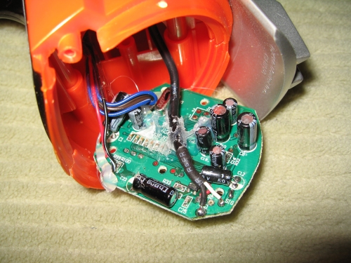
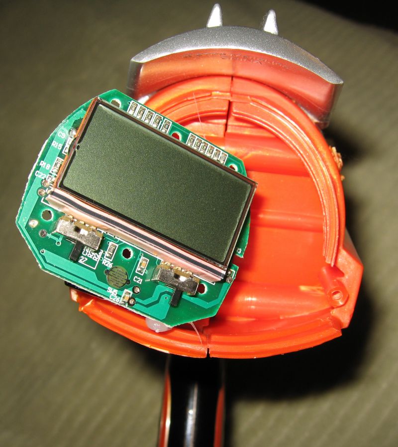
The radar gun has its own ATmega88 which receives an ADC input from the waveguide, translates it into velocity, and drives an LCD screen. When the trigger of the radar gun is pulled, the waveguide is activated and velocity is updated on the LCD screen every second. When the trigger is released, the ATmega88 displays the highest velocity seen during the triggering. Chuck advised me that the best place to tap into the radars velocity measurements was at the ADC input of its own MCU. The signal there has undergone mixing with the transmitted signal, and our hypothesis was that it would be a voltage proportional to velocity. This signal could be fed directly into our own ADC input and interpreted into rain. The PCB inside the radar gun houses its ATmega88 and LCD on one side and most of its other components on the other. Chuck pointed out that the factory included a test point for the ADC input to the ATmega88, a small thru-hole that could be easily accessed from the non-MCU side (turning the PCB over and working on the ATmega88 side required removing the magnetic-strip-connected LCD, a very intrusive and risky maneuver). So, a wire was soldering to this test point, as well as to the guns ground. This wire went to our own ATmega644s ADC5 input, and the ground to the general ground of our circuit. The figure below shows the test point, ground, and trigger wires on the non-MCU side of the radar guns PCB.
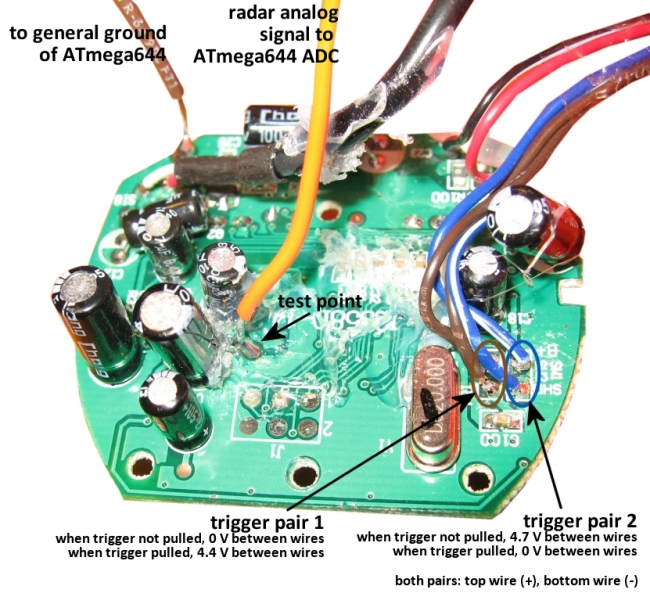
Triggering the radar gun was a tricky process. The figure above shows the voltages on each of four trigger wires coming from the guns trigger. These voltages were used to determine what signals (on or off) we had to send in order to simulate a physical squeezing of the trigger. The guns trigger has two switches. One of them is normally closed, and connects the guns circuit to ground through a 330K resistor. The other one is normally open, and when it is closed by physically squeezing the trigger, it enables three 5V regulators that power the digital circuitry, amplifiers, and ADC converter input. After many failed attempts at turning on the gun electronically, the final solution was to unsolder the bottom brown and blue wires in the figure, and connect them to outputs from port B of my own MCU through 1k resistors. To turn on the gun, we send a 1 to the blue wires pad and a 0 to the brown wires pad. To avoid having the gun stay on indefinitely, just as important was to send a 0 to the blue pad and a 1 to the brown pad when turning off the gun. These signals must be maintained for at least 20 seconds (the shutdown time of the radar gun as it shows the maximum velocity read), or else the gun with stay on indefinitely. This was the biggest problem of triggering and remains a limitation of the design; the outdoor unit must not be turned off immediately after the radar readings are taken, or else the gun stays on and drains the batteries.
Several problems were encountered while hacking into the radar gun, the foremost of which were an unreliable zero voltage of the test point and a hyper-sensitivity to velocity. In the end, the test point measures 525 mV when seeing zero velocity and increases up to 700 mV with hand waving and other motion. After much variation, the baseline ADC reading of the test point settled at 120. When the gun is pointed in the air and there is no motion in front of it, the ADC input consistently reads 120. With rain pouring from a funnel positioned 1 meter above the gun, this value fluctuates rapidly, increasing to approximately 135. The still-functioning LCD readout of the radar gun was used to associate these ADC readings to velocity. The ADC readings were cascaded at a 1 ms sampling rate through a serial connection to HyperTerminal, and water was poured at the gun as the LCD velocities were examined. Deviating a little from the initial expectation of 5mph (calculated above), the droplets reliably measured 8 mph. Interestingly, the voltage of the test point seemed to be proportional to radar cross section rather than velocity, since waving my hand in front of it sent the ADC voltages flying to 200+ while rain drops only registered at 135. The LCD-displayed velocity of my hand barely exceeded 4 mph, however, while the rain was clocked at 8 mph. For this reason, the initial plan of categorizing rain according to velocity was abandoned in favor of a simpler rain-detector. For the purposes of our demonstration, we decided to be satisfied with a rain or no-rain decision by the radar gun. A limitation of the setup is that there cannot be any motion in a 20-degree line-of-sight cone coming from the gun, or else it will be interpreted as rain and lead to a false alarm. This may be hard to ensure in the lab demonstration, but in an actual outdoor implementation, the apparatus can be positioned such that movement above the gun will be unlikely.
Homemade Anemometer
The anemometer is a homemade design fabricated at minimal cost using readily available low tech components. The design concept is called an 'Easter Egg' anemometer because it uses toy plastic Easter eggs for the rotating wind impeller as described in the references below.
As for any mechanical device employing rotating parts, the design challenge in the low cost anemometer design is one of friction and balance. Several of the design concepts recommend using discarded computer hard drive assemblies for the sake of the frictionless bearings. Since a discarded hard drive was not immediately available our design relied on simple homemade bushings fabricated from PVC pipe components. The rotating hub was fabricated from two circular plastic electrical outlet box covers laminated over the three propellers. The plastic hub halves were grooved to fit three brass rods used for the propellers oriented at 120?. The two hub halves were then glued together over the propellers. For both the rotating hub and shaft bushings the critical design consideration was accurate centering of the propeller shaft to ensure balance. In order to reduce friction a spray Teflon lubricant was applied to the load bearing points. The simple anemometer assembly is shown in the figure below.
The anemometer uses a DC motor operated as a DC voltage generator when reverse driven by the rotating propeller shaft. The voltage generated is proportional to the shaft rotation rate which is proportional to wind speed. The anemometer output voltage was calibrated to wind speed using the following calibration procedure. The anemometer was mounted vertically on a vehicle driven as the speedometer readings were noted on a relatively windless day. A voltmeter was attached to the DC motor leads and the output voltage recorded as a function of vehicle speeds from 10 to 30 mph in 5 mph increments. The readings were repeated at least four times with the vehicle driven in varying directions to allow for residual ambient wind. The results of the anemometer calibration test are shown in figure 2 below.
Humidity
The humidity measurement is not from a voltage outputting sensor like the others. It is a capacitor that changes its capacitance (330 pF ~ 55% relative humidity) based on humidity. This required the technique used in Lab 1 to measure capacitance. The following circuit was used, the same as in Lab 1 except a 100k resistor is in place of a 10k resistor to account for picofarads instead of nanofarads.
Port B3 is set to an input, then port B2 is made an output and discharges the capacitor through 100 ohms. B2 is then made an input and a timer is started as the capacitor begins charging. We determine the time it takes for the voltage on B2 to reach that on B3, using the timer1 input capture function triggered by the analog comparator.
Solar Panels
Our project uses two Sun Power PWR1241 photovoltaic solar cells. Each outputs 4.5 V at maximum insolation, with a maximum current of 90mA. Two of these in series are perfect for charging a 4.8 V collection of AA NiMH rechargeable batteries. We use the technique of Abigail Krich, in her final project, Self-Powered Solar Data Logger of Spring 2006. She uses a BUZ71 transistor to regulate the charging of the batteries. Her project has a separate photodiode sensor for sunlight intensity to provide maximal accuracy, but we use the voltage across the same two panels as a rough estimate of sunlight intensity. The original plan was to use a shunt resistor to measure the current through the solar panels, since current varies more closely with intensity. When we acquired the panels, however, the voltage across them was remarkably reactive to sunlight, so we decided to use an ADC input to directly measure voltage. We measure the battery voltage as well through a 11/1 voltage divider. When it is dark or the battery is fully charged, we disconnect the solar panels from the circuit and are only used to measure sunlight intensity. The figure below shows this circuit, as well as the other ADC inputs and port B triggers.
A Mega644 protoboard, designed by Bruce Land, carried the outdoor microcontroller. Another small solder board carried the LM34 temperature sensor, humidity circuit, solar switching circuit, and machine plugs for inputs coming directly from the wind gauge and radar gun. This solder board is considered the brains of the outdoor weather station because it brings together the sensors and the MCU. Another peripheral attached to the MCU (through the solder board) is the transmitter, which (at the suggestion of Bruce) was creatively mounted on half of a small solder board with an upside-down MCU socket on the other side.
As an added bonus (which may have been more work than it was worth), all of the inputs and outputs are hardwired to STK500 ribbon cables in addition to the loose input and output wires intended for the protoboard. So, the main solder board has several wires labeled A0, A1, A2, etc, that plug into a row of 15 machine plugs on the protoboard, along with an additional two blue ribbon cables with all of the I/O wires duplicated to go to the STK500. It was a lot of work to duplicate the inputs and outputs to easily convert to STK500-mode, but it was very useful when testing the weather station to have serial outputs for the sensors. Oftentimes, a given weather condition was being displayed graphically on the LED matrix and we wanted to know why.
Physical Structure
Housing for the outdoor unit was needed that would protect it from the elements. A perfect enclosure turned out to be a tupper ware material cereal storage container. It inherently tilted the radar gun a slight 20-degree offset from vertical, great for intercepting the rain drops falling from the funnel one meter above. To hoist the funnel above the radar gun in such a way, we used scavenged PVC pipe with couplers and elbows to build a tower. At the top of the tower, the DC motor anemometer assembly fit perfectly, and a T-joint extended the funnel just in front of the radar beam. This setup is shown in figure below.
Outdoor Weather Station Software Design
The code for the outdoor weather station can be found in Appendix A. It consists of seven tasks, each in charge of a different sensor and the last in charge of transmitting. The code is intended to be as adaptable as possible, with all of the important timing definitions at the top for easy access. The program is centered on the ADMUX. In the initialize method, aside from setting up the usual timer0 1 msec timebase, we initialize the analog-to-digital converter for heavy use later on. For now, we use the ADCSRA register to enable the ADC, start a new conversion (for the first measurement, temperature; first ADC reading is thrown out), clear the interrupt flag and disable auto triggering (it does not use either of these features), and set the prescalar to produce an ADC clock rate of 125 kHz. Also in initialize, the ports are set up. The program only uses port A and port B (not counting the prototype boards built in LED, port D.2, to indicate a transmission). All but two of the ADC inputs of port A are used, and port B is used for triggering and other miscellaneous tasks. The following is an I/O summary, categorized by sensor:
| Temperature | ADC7 |
| Humidity | B.2 and B.3 |
| Solar Panel | voltage output, ADC2 Battery voltage, ADC6 BUZ71 gate, B.7 |
| Wind Gauge | (+)ADC1, (-)ADC0 (x10) |
| Radar | ADC5, B.6 trigger, B.5 off trigger |
| Transmit | B.1 Data, B.0 Valid Tx (VT) |
The program is a sequence of events, all executed in specific order by main(). A series of timers controls the overall execution of tasks. Although they are not used by the weather station when disconnected from a computer, UART fprintfs are scattered throughout the program to display weather readings if connected to an STK500. This is useful for testing, or if a certain threshold for one of the weather conditions is too low or high.
Main begins by starting the conversion for the first of six sensing tasks: temperature. The variable wait is the primary time counter; main always checks that wait has gone to zero before executing a new task and resetting wait. Each task is associated with a certain *task*_done signal. When the temperature task is complete, for example, it asserts temp_done to tell main (along with wait = = 0) that it should execute the next task, humidity. Main first checks the variable sending_done, because it is the last task in the sequence, and it knows to restart the cascade with the temperature task if sending_done = 1. Wait is typically set to either measurement_interval, the time between each measurement (1 second), or data_interval, the time between each collection of measurements (40-60 seconds, depending on desired checking rate; would be around five minutes if used continuously, in real life).
The ADC uses a reference voltage of 1.1V for every conversion. This turned out to be perfect for the low voltage sensors like wind (maximum 30mV), radar (always just above or below baseline of 525 mV), and temperature (10mV/degree F). It is also suitable for reading solar and battery voltages through an 11-to-1 voltage divider, which takes their 9V and 4.8V maximums, respectively, down to below 1.1V. Wind is the only sensor to use a differential gain channel of the ADC, with 10x amplification bringing it to a moderate value on the 0-1.1V scale.
The temperature task simply reads in the value on ADC channel 7 and multiplies it by a coefficient to get temperature in Fahrenheit. Although adjusted empirically, the coefficient for every conversions follows the form: Vin = (ref voltage / 255)ADC
It makes the first of five transmission decisions according to the code described in the indoor display section. It categorizes the temperature into four levels and sets two bits to this level for later transmission. Also in temperature(), the radar is triggered using ports B.5 and B.6 because the radar voltage takes some time to settle down when it is first turned on. When temperature finishes, main() waits until measurement_interval is over before executing the next task, humidity. Lab 1, capacitance measurement, is entirely contained within this task and the surround ISRs. The timer1 overflow and capture ISRs determine when the voltage on B.3 reaches that on B.2. The humidity is a relative figure, so it is kept as a capacitance (in picofarads) instead on converting to rh %. We chose thresholds for our humidity decision empirically, based on the humidity in the demonstration room and the need for a demonstrable change in humidity. Each task from now on begins the ADC conversion for the next one, so humidity starts the conversion for sunlight intensity.
The solar task reads in ADCH and multiplies it by solar_coeff to get voltage. For the demonstration, however, we chose our thresholds empirically based on the raw ADCH readings. Again, we make a sunlight decision for transmission, categorizing the sunlight in four levels: night, cloudy, moderately sunny, and very sunny. These correspond to 00, 01, 10, 11 when transmitting to the indoor unit, which changes its condition intensity bar accordingly.
The next task is important for the solar recharging circuit, because it measures the battery voltage and connects or disconnects the solar panel when appropriate. The battery ADC is read and converted to volts. If it is below 4.6 V and there is enough sunlight, the panel is connected by turning on port B.7. To avoid overcharging or discharge into the air through the solar panel at night, the panel remains disconnected in both of these cases.
The wind speed measurement is the first of two extended measurements. In order to get an accurate measure of wind, several ADC conversions are done on the incoming voltage from the rotating anemometer. The duration of this task can be adjusted with windONlength in the definitions, but it was 15 seconds for the demonstration, with an ADC conversion every half second. The wind task also categorizes the wind, but it is harder now that there are more than just one ADC value to compare. The task counts how many conversions fall into each of four categories: no wind, low, moderate and high wind. Then, it concludes the level of wind is the one with the most number of conversions. As discussed in Hardware above, our wind meter is calibrated such that mph is exactly equal to mV output.
Finally, and most dramatically, the radar guns voltage is measured in the radar task. Whereas the wind program could afford to run a conversion every half-second, the radar voltages are essentially instantaneous and the radar consequently runs one conversion every millisecond. Since the baseline (zero velocity) ADC reading is 120, and a rain drop pushes that up to around 130, any readings above 125 are considered to be evidence of rain. If enough conversions fall above that threshold (which can be adjusted at the top of the program depending on desired sensitivity), the task concludes that it is raining. If too many false alarms are occurring, either the 125 threshold or the required number of such readings can be adjusted upward. Unlike the other tasks, which make transmission decisions by categorizing their intensity, the rain task is a binary decision and has room for creativity. Here, our two-bit code tells the indoor unit to display one of: a meadow scene, a rain scene, an ice scene (rain + low temp), or a rainbow scene (rain + bright sun).
The final task is the most important because it sends all of this information via the Holtek/Reynolds Electronics TXE-418-KE encoder/transmitter module. This unit, along with its receiver counterpart, were sampled from Reynolds Electronics, who combined the Holtek encoder with their own transmitter. This made transmitting a simple matter of asserting the transmit enable (TE) bit while the appropriate data is on the D0 line. A pinout of the transmiiter is shown below. The address lines A0-A9 must be the same on the transmitter and receiver for communication to occur. A2 was hard coded to ground and the rest were left floating.
These modules are capable of sending 8-bits per transmission, but because of the limited number of available inputs on the indoor MCU, we send one bit at a time. Our code is a sequence of 10 bits, and the send task runs through a for-loop to transmit them one at a time. The send rate can be adjusted (tx_length), but it is set to 400 milliseconds so the receiver has ample time to recognize a transmission.
Results
Speed of Execution
The measurement interval of the Weather Canvas outdoor unit can be customized depending on the time accuracy desired. In a real life implementation, one would probably not require measurements more than every minute or even every five minutes. The weather shifts between extremes, but it never does so within a five-minute span. The measurements can also be decoupled from one another, so temperature and others can be taken virtually continuously while the more battery-intensive radar rain gauge only checks in every ten minutes. The radar sampling rate itself is a more important factor. In the demonstration, it was sampling the voltage on the ADC channel every millisecond, looking for evidence of rain. In reality, the radar is pulsed to spend 25 microseconds on, 75 microseconds off, which is way below the ADC clock rate. Many of the rain drops, therefore, are missed by the ADC because they occur between samples, but 1 millisecond intervals are enough to catch the voltage residue from most drops, if not sometimes the peaks. Finally, transmission is occurring at a rather slow rate of one bit per second to ensure full reception inside. There is no need for this to be faster, since there is not a backlog of data, but it could be much faster with an increased risk of lost bits.
The program controling the LED matrix requires a high update speed, since any flickering in the LED matrix would be unacceptable. Luckily, the microcontroller is fast enough to handle controlling 32 pins as well as RF decoding at a high enough rate so as to not produce flicker. This was not the case when we attempted to use ideal parameters, as discussed in the indoor software section. When the PWM period was set to the ideal value of 255, flickering ensued, and by experimentation a period of 64 (256/4) was found to be an acceptable tradeoff, still producing a superfluous number of colors. It should be noted that this is a software period, and does not directly correspond to a time measurement because a software period can vary depending on the number of computations involved. But since so much flickering is visible, this corresponds to a time period of much less than one-sixtieth of a second.
Accuracy
The Weather Canvas actually gathers much more accurate information than can be displayed on the LED matrix. Its sensors are capable of tracking weather conditions with the potential for highly scientific applications. The anemometer, for example, has a precision of 1 mph, and with mV directly proportional to mph, it continues to agree exactly with car speeds and known wind speeds.
The radar rain gauge does not measure inches of rainfall, but it is perfectly suited to this application. It is sensitive to raindrops greater than 1/4 in size, and can detect the presence of just a few drops. The velocity of falling rain drops has never been tracked before, and an inexpensive radar gun is actually the optimal one for the job. More powerful military radars are designed to look past obstacles like rain drops for more significant targets, but the Hot Wheels Radar Gun has so much smaller gain that it is looking for the slightest Doppler shift in the returning signal, and that includes rain.
The LM34 was used to take temperature reads and as stated in the datasheet it has a temperature accuracy of approximately +/- 0.8 degrees Fahrenheit around a temperature of 77 degrees Fahrenheit, which is typical of Ithaca in spring and early summer. In the winter, the accuracy drops to around +/- 1.0 degrees Fahrenheit at 0 degrees Fahrenheit, which is more than acceptable for our display system.
Conclusion
Most of the components fit into the overall design exactly as anticipated. One notable exception is the temperature sensor. After transferring our project from the STK-500 to our prototype board for the outdoor unit (which operates at a maximum Vcc of around 3.2V from the rechargeable battery system), we found that this voltage is sufficient for all components of the sensor circuit except the LM34 temperature sensor. After much debugging, we glanced again at the datasheet and discovered that the minimum Vcc it can produce results at is 5V. This required the use of a separate voltage supply for the temperature sensor at the last moment, a 9V battery-powered auxiliary sensing module. This actually helped for demonstration purposes because it gave us more access to the temperature sensor, but we would have rather had all the components running from the same, renewable source. If we were to do the project again, we would choose a temperature sensor with a lower minimum supply voltage.
After the LM34 debacle, we found that the rechargeable battery concept had bigger problems than the inability to power the LM34. The NiMH AA batteries each have a voltage of 1.2V, 0.3V lower than the output of alkaline AAs. This means that fully charged, they can only generate 4.8V, which is already lower than the typical Vcc for our MCU. Furthermore, we found that the reliability of our transmissions was suffering when their voltage fell below 4V. The transmit signal began flickering and fooling the receiver into thinking two separate bits had been sent. When the batteries lost charge below 2V, the protoboard was no longer programmable. In the end, only a short time range existed in which the 4 NiMH batteries successfully powered our circuit. To ensure a successful demonstration, we disconnected the solar charging wire from the batteries and used a 9V alkaline battery with a regulator, instead. In doing so, we also regained the use of the original LM34. The framework for solar charging remains in our circuit, but the choice of battery voltage needs to be improved if the outdoor station is to last through a sunless night.
FCC Considerations
Our RF system operates at 433 MHz, which is an unlicensed band of the frequency spectrum, and we do not have any plans to produce the unit commercially, so we are in compliance with FCC frequency regulations. In addition, according to the organization Epilepsy Ontario, the triggering of a seizure via flashing lights occurs between 5 Hz and 30 Hz. The LED matrix refreshes at a much higher rate, so we do not see any potential for frequency-induced seizures. Finally, since all of the components used in the design are Commercial Of-The-Shelf (COTS), we can foresee no additional safety violations.
Our design for the solar recharging circuit was based off of Abigail Krichs circuit in her Spring 2006 ECE 476 final project, a self-powered solar data logger. The modifications made to the Hot Wheels Radar Gun could be done without permission because it was for academic use, but we would not be able to sell the Weather Canvas or claim it entirely our own because a whole component is made by Mattel. They intend the Radar Gun to be used in the way it was intended, although the preponderance of projects hacking into it on the Internet lead us to suspect a large share of its users are immediately looking inside.
IEEE Ethics Considerations
Our project adhered to the IEEE Code of Ethics at all times. There was never any danger to other students or faculty from any side effects of our project. All of our collected data is genuine, with no manipulation of information to make it appear as though we had progressed farther than we actually had. Our understanding of microcontrollers, especially in the areas of PWM, RF communication, and analog-to-digital conversion, was increased dramatically (as well as our ability to multitask and prioritize). All intellectual property from others is properly credited in the references section. We were very careful to be considerate of others in the lab environment, stepping softly in the late hours and being cautious so as to not accidentally step on any groups work.
Appendix A: Code Listings
RGB LED code performing PWM to illuminate dots
Outdoor weather station sensing program
Appendix B: Schematics
Diagram of Outdoor Weather Station (above)
Appendix C: Cost Analysis
|
Part |
Quantity |
Unit Cost |
Total Cost |
| RGB LED 8x8 Matrix (YSM-2388CRGBC) |
1 |
$12.00 |
$12.00 |
| Linx Technologies TXE-418-KH (encoder/transmitter) |
1 |
Free Sample |
$0.00 |
| Linx Technologies RXD-418-KH (decoder/receiver) |
1 |
Free Sample |
$0.00 |
| LM34 Temperature Sensor |
1 |
$1.95 |
$1.95 |
| PWR1241 Sun Power Solar Panel |
2 |
$3.20 |
$6.40 |
| 12V power supply |
1 |
$5.00 |
$5.00 |
| NiMH AA 1800 mAh rechargeable batteries (4-pack) |
1 |
Ultimately Did Not Use ($9.00) |
$0.00 |
| 9V battery |
1 |
$2.00 |
$2.00 |
| 9V Battery Clip |
1 |
$0.75 |
$0.75 |
| Prototype Board |
2 |
$4.00 |
$8.00 |
| Mega644 PDIP Package |
2 |
Free Atmel Sample |
$0.00 |
| SIP/Header Socket |
100 |
$0.05 |
$5.00 |
| Mega644 socket |
4 |
$0.50 |
$2.00 |
| Small solder board |
3 |
$1.00 |
$3.00 |
| Humidity sensor (480-2903-ND) |
1 |
$4.82 |
$4.82 |
| Hot Wheels Radar Gun |
1 |
$10.00 from eBay |
$10.00 |
| PVC Pipe and Elbows |
1 collection |
$3.00 |
$3.00 |
| Cereal tupperware enclosure |
1 |
$1.50 |
$1.50 |
| DC Motor, shaft |
1 |
Prior ownership |
$0.00 |
| Shadow Box |
1 |
Prior ownership |
$0.00 |
| Nuts and Bolts for Tower |
4 |
0.10 |
$0.40 |
| Wooden Base |
1 |
Free from Home Depot |
$0.00 |
| Dinosaur Eggs |
2 |
$0.25 |
$0.50 |
|
Total Project Cost: |
$64.32 |
Appendix D: Work Split
The Weather Canvas was easily divided between the indoor LED display and the outdoor weather station. Michael worked on the indoor display, while Charlie did the outdoor unit. We came together to do RF communication between the two, and then jointly debugged the entire design.
References
Chuck Baird's Hot Wheels Radar Gun Project
Hacking the Hot Wheels Radar Gun by Ed Paradis
Easter Egg Anemometer
Homebuilt anemometer
Building an anemometer
Homemade Easter Egg anemometer
Self-Powered Solar Data Logger By Abigail Krich
RGB LED Datasheet
TXE-418-KH transmitter datasheet
RXD-418-KH2 receiver datasheet
STK 500 User Guide
Acknowledgements
Thanks for all the help of Bruce and the TAs! We learned more in this class than any other.