"A 3D canvas on which the artist can draw using trilaterated coordinates from ultrasonic delays."
Project Soundbyte
For our final project in ECE 4760, we designed and implemented a three-dimensional paint program consisting of hardware, a microcontroller, and a PC running MATLAB. All three modules strongly interacted to allow the artist to wave a pen around in space and see their movements translated in real time to various projections on the computer.
An ATmega644 microcontroller calculates the time delay from the pen to three known points and communicates these values continuously to a PC running MATLAB via a serial port. MATLAB then translates the delay information to real xyz-coordinates and displays the data in various forms on a fully functional GUI. The artist can additionally use the pen as a camera to look around the design space.
We wanted to create this system as a facilitator of creativity. Because of the strong relationship between the artist and the medium, we hoped that a new take on the canvas would instigate new creative processes. This idea encouraged us to create a device as simple as possible so that as little technological bias would be injected as possible.
High Level Design top
Overview
When contemplating ideas for final projects, we decided to rigidly follow a set of specific stipulations. First, we wanted to implement something new that would be a genuine joy to use and build rather than implement something just because it was technologically difficult and would satisfy the requirements of the class. Because this project is often thought of as the culmination of a Cornell ECE’s undergraduate career, we wanted to build something that relied on many aspects of our education: physics, mathematics, analog and digital circuits, signal processing, microcontroller programming, peripheral communication, and high-level coding to name a few.
The original idea was to design a system for tracing out 3D objects so that someone could, for instance, take a pen and trace out a coffee mug and then build a 3D model out of it in a computer for use in animation or finite element modeling. Physical limitations quickly took effect, however. Because you would rarely have line-of-sight between receiver and transmitter due do whatever object you were tracing, you would need to communicate via radio waves. We searched for possible ways to accurately measure distances based on this, including via the amount of power received between an RFID tag and reader, but to our knowledge distances have only been accurate with this method to around 10 cm, which is far outside acceptable bounds for the application. Our research yielded no way to proceed with RF using relatively simple hardware, so the natural progression of this idea was to remove the object being traced.
By removing the object, it was now possible to maintain line-of-sight between Rx/Tx pairs at all times. The idea was now simply a 3D paint program that had a plausible implementation through high frequency sound and the known propagation delay of acoustic waves to trilaterate distances.
With this core idea in place, ideas bloomed for how to make the system fun to use. By interfacing with MATLAB we could display the drawing in high quality plots that were perfect for exporting. Further, MATLAB supports full GUI design, so we could make a nice interface for the artist to select various brush sizes, colors, and styles. Bruce Land also suggested we have a stereoscopic representation of the drawing. To make the drawing process more fluid, we decided to have the program operate in a ‘paint’ mode to draw or in a ‘camera’ mode in which the artist could use the pen as a virtual camera to look around their drawing.
Mathematical Background
The foundation for the device relies on the fact that the speed of sound is constant in a given medium. Under everyday conditions, the speed of sound in air is 340.29 m/s. This means that we have a bijective mapping between time and distance for sound propagation. By emitting a sound pulse and recording the time delay between emission and detection, we calculated a displacement via the following equation:

One delay measurement will give you a position in one dimension along the line-of-sight of the transmitter and receiver, yet in three dimensions all a single delay value will tell you is that the emitter was somewhere on the surface of a sphere centered at the receiver and with a radius equal to the time delay multiplied by the speed of sound. To determine a true xyz-coordinate, we needed to get more delay measurements. Positioning another receiver uniquely will give you two spheres of possible locations centered around each receiver, and the two sphere’s intersection (generally a two-dimensional circle) will give you all the possible locations that satisfy both delay measurements. Adding yet another unique receiver will further stipulate the position of the pen, but this time exactly. The resulting coordinate system and placement of the three receivers can be seen below.
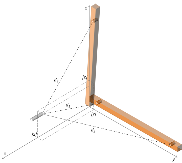
Mathematical coordinate system for trilatertion
We now have three equations (spheres located around each receiver) and three unknowns (where l is the displacement of each receiver along a given axis), thus a single unique position for the pen can be determined.
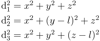
Three sphere equations
Solving this system of equations can be tricky, but noticing that some equations can be subtracted from one another greatly simplifies calculation. The z and y coordinates can be calculated directly from the delay measurements, and then using these values x can be solved for. You end up with the following:
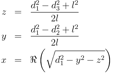
Trilateration equations for our setup
Note that we are taking the real part of the square root in the x calculation. If our delay measurements were mathematically perfect this would be an irrelevant calculation because the square root argument would never be negative. However, because the data is imperfect it is certainly possible for the square root to produce imaginary results. Taking the real part is a very good approximation given the imperfect data, however. These equations allow us to perform what is called a trilateration.
Logical Structure
There were three primary components involved with the system: the microcontroller, the hardware, and the PC running MATLAB.
The microcontroller’s primary function was to facilitate the rapid acquisition of time delays between the transmitter and three receivers. This job was tasked to a microcontroller because of its inherent ability to interface with analog hardware and communicate with higher-level machines like a PC. The microcontroller coordinated the emission of a sound pulse according to many timing specifications. For instance, it could not emit too fast or the receivers would become confused as to which received pulse corresponded to which emitted pulse. Additionally, some receivers might not have received a pulse if the pen was directed away at too great an angle so it needed to be prepared to handle measurement timeouts. The microcontroller was responsible for keeping all pulses and receptions locked in step to ensure quality data. Originally the microcontroller was not tasked with any signal processing requirements, yet this job was also later assigned to it to improve responsiveness. The microcontroller was also to follow a protocol to transfer data up to MATLAB. When MATLAB requested data, the microcontroller was to respond via UART serial communication with a packet containing information relating to the pen’s status (button pushed or not) and the three delay values.
The hardware was further broken up into two components: emission and detection. The microcontroller produced a 40 kHz square wave suitable for the ultrasonic Tx/Rx pairs we used. However, the microcontroller could not generate signals sufficient enough to properly drive the transmitter (it could handle 30 V peak-to-peak values but the ATmega644 was limited to 5 V peak-to-peak output). Thus, the 40 kHz signal required significant gain to maximize the strength of acoustic pressure waves and therefore maximize directionality (wider is better), possible distance from receivers, and signal-to-noise. Further, hardware was responsible for providing the artist with an easy way to specify whether or not they wanted to be painting a stroke at a given moment. This was accomplished via a button mounted on the pen (so it was collocated with the transmitter). On the reception side the hardware had to gain the received voltages such that they were interpretable by the microcontroller.
MATLAB was where the bulk of the artist interaction was centralized. It was to produce a fully functional GUI so that the artist could change various parameters about the paintbrush (i.e. color, etc.) and receive visual feedback as to what they were drawing. MATLAB was to provide a variety of options for how the feedback was displayed (3D plot, 2D orthogonal projections, etc.). MATLAB needed to request data from the microcontroller and parse it into xyz-coordinates via the trilateration equations above. It also needed to parse the state of the push button to determine whether or not to draw a stroke. When the artist was not drawing, MATLAB was still to display a cursor of the current location of the pen. When the program was in ‘camera’ mode MATLAB was to interpret the pen position as the location of a camera so that the artist could look around their drawing. Further, MATLAB had minimal signal processing requirements to further smooth the data. Finally, MATLAB needed the ability to export the drawing as a jpeg.
High Level Block Diagram

High-level block diagram.
Hardware and Software Trade-offs
Our design philosophy was to simplify the device as much as possible so as not to impede upon the artist’s work-flow. To this end, we designed the system with minimal hardware UI and instead concentrated the UI in software. Accordingly, we implemented the pen with a single critical button to indicate drawing or not drawing. The button was located toward the front of the pen so that the artist could hold it and press it only when they wanted to make a stroke. Obviously, having software UI for this function would be comparatively cumbersome. For the rest of the UI, we could have used hardware buttons or toggle switches but software seemed a more appropriate choice. We wanted to limit the physical footprint of the device, and running a bunch of wires to and from physical buttons seemed unnecessarily complex for something like selecting the brush color. Putting these sorts of options in hardware also meant that the microcontroller was responsible for capturing and relaying button states up to MATLAB. This was inefficient a) because the microcontroller did not need to know the button states and b) because it would waste cycles and time to capture and transmit them (UART communication is very slow, so data should not be sent unless it is absolutely necessary). Further, implementing these options in software made the program much more extensible: new features could simply be added in code without any new hardware development.
The rest of the hardware/software breakdown was predicated entirely by the limitations of hardware and software and thus didn’t require a strategic breakdown.
The MATLAB/ATmega644 break down was a harder line to walk. Initially we only wanted the 644 to record delay information and send it up so that it could run as fast as possible. However, we quickly discovered that one of our greatest bottlenecks was how quickly MATLAB could process a given delay packet, put it out on all plots, and update the cursor position. So, it happened that the ATmega644 could produce delay information much faster than MATLAB could read it. Because MATLAB was originally doing the DSP operations, this meant a fairly substantial delay (~500 msec) from physical movement to display on the GUI because of the time it took for new data to fill up the sliding window buffers used for processing. To fix this, we off-loaded the signal processing to the microcontroller, which meant that the MATLAB code would instead receive already filtered data, and the responsiveness of our system increased tremendously.
Standards
Given the relatively simple hardware involved in this project, few standards were used in implementing communication between the PC and the peripheral device (MCU). Serial communication between the MCU and the PC made use of the MCU's onboard universal synchronous/asynchronous receiver/transmitter (USART) peripheral unit and took place via the STK500's Serial port and PC's USB port. As it was only used asynchronously, it may be referred to as a UART. This UART was used in conjunction with the RS-232 communication standard.
Intellectual Property (Patents, Copyrights, and Trademarks)
We chose to name our completed product 3D Paint, which may potentially infringe on the Paint trademark held by the Microsoft Corporation for its own graphics painting program. If this becomes an issue, we can opt to change the name of our product.
We do not believe that the technology infringes on any existing patents. In Relevant Patents, we have linked a number of patents relating to ultrasonic three-dimensional positioning systems. There is also another student project for ECE 4760 from Spring 2009 (UltraMouse 3D by Karl Gluck and David DeTomaso), which makes similar use of ultrasonic sensors for three-dimensional positioning, but only accurately records two-dimensional coordinates. However, as our design uses different methods to detect pulses and filter data, we do not believe that we have violated any of them.
Software Design & Implementation top
The software was implemented across two platforms: the ATmega644 and MATLAB.
Microcontroller
The microcontroller code was written to be as straightforward as possible. It operated within a while(1) loop after some basic initialization procedures. Initialization procedures included setting up UART communication (we used a baud rate of 38500 to speed up communication), configuring i/o pins, initializing timers, setting up interrupts and initializing variables.
The code required the use of all three timers provided by the ATmega644. We used timer0 to establish a .5 msec time base from which we could dispatch various actions (like initiate a new pulse train or signal a timeout). Timer1 was used as a means to calculate the delay in cycles that it took for a pulse to be detected. Because we wanted to time as accurately as possible, timer1 was counting at the full clock speed (16 MHz) of the MCU. This corresponded to a range resolution of roughly 21 μm, which was more than acceptable for the purposes of the system. Timer2 was utilized to generate the 40 kHz square wave required by the ultrasonic Tx/Rx pair.
Five interrupts had to be written for proper operation of the code. First was the timer1 overflow interrupt. This interrupt was triggered every time timer1 (an 8 bit counter) overflowed. Because 8 bits was not nearly enough space to represent a typical delay time in cycles (they were generally on the order of 10,000 cycles), we simply had the overflow interrupt increment a variable by 256 every function call so that we could keep track of the true cycle count. The second interrupt ran whenever we received a new character on the serial port. This was used to indicate to the program that MATLAB had sent a command and that the 644 would need to respond. The other three interrupts were hardware interrupts on int0 (pin D.2), int1 (pin D.3), and int2 (pin B.2). Each ultrasonic Rx was wired up to a given pin after gain, so the interrupt would fire when the pulse was received. This allowed us to stop the timer on the delay count. There is an alternative way to do this, and was implemented in the ‘3D Ultrasonic Mouse’ project for ECE 4760 by Karl Gluck and David DeTomaso. They had an interrupt fire periodically at 160 kHz and poll the receivers for an acquired pulse. We felt better about the interrupt-driven scheme because of the innate aperiodic nature of the pulses coming in. Polling at 160 kHz automatically limits your resolution to 2 mm, whereas our scheme imposes no set limitation on resolution. Obviously, the drawback of the interrupt method is interrupt collisions, or when two or three receivers receive a pulse all at the same time. We tested this, and found that for this worst case scenario it took roughly 100 cycles to get in and out of a given interrupt, implying a maximum error of 200 cycles if they all interrupted at exactly the same time. While this maps to an error of 4 mm, it is only for an extremely small subset of the drawing space where the pen is equidistant to all receivers. For the overwhelming majority of the space, however, we saw a negligible error using the interrupt method.
After initialization the code entered a while(1) loop and constantly checked a number of conditions. First it updated the state of the pen button, which was fully debounced, every 20 msec. The button debounce code was written by Bruce Land and was provided on the 4760 course webpage. The button debounce code had a variable containing the current state of the button (i.e. pushed or not pushed). This variable was what was sent to MATLAB to indicate whether or not the artist was drawing.
Next the code checked whether or not it was time to emit a new pulse. We set the inter-pulse period (IPP) to 20 msec for this lab to ensure that any reflections from previous pulses would have plenty of time to die out before we began a new measurement. This corresponded to a distance of roughly 6.8 meters, which was plenty in practice. If it was time to emit a new pulse train, we reinitialized all timing variables and also rearmed the interrupts. By rearming, we mean that each interrupt would only record a value if it were armed. This prevented a lot of misfiring and ensured a given receiver was not constantly retriggered while waiting for one of the others to trigger. We also only emitted a pulse for .5 msec. This was all that was necessary to properly trigger the receivers, and going any longer than this would potentially confuse the receivers when operating in steady state. Limiting the length of the pulse helped to keep the environment quiet for each pulse. The loop also checked for a potential timeout. If all three receivers had not been triggered within 7.5 msec (a distance of 2.5 m) then the system would reinitialize everything, throw out the bad data, and emit another pulse. This was to guarantee that any data that was captured came from one unique pulse.
The loop also checked for whether or not all three receivers had triggered. If they had, it entered them into the signal-processing buffer. We converged on a two-stage processing scheme for this project. First we performed a sliding window median filter. The median filter was a crucial first step because it was possible for there to be very large outliers compared to the true delay. These were most often caused by pulses that reflected and triggered a receiver after the system had already reinitialized and sent out a new pulse. Median filters were preferable to some type of low pass average filter because the large outliers would still put huge skews in the data if averaged, but be completely removed if mediated. There were a few implementation challenges to getting the median filter working. First, we wanted to create a buffer that would take the median of the x most recent delay samples. To do this, we created an index to an array that would cyclically drop samples into the buffer. We first placed the sample at index 0, then index 1, and so on all the way up to index x-1, where it would modularly roll back to 0. This made it so that we didn’t need to move any values around in the array when a new sample came in. Next, we needed to sort the data (as this is typically the most efficient way to find a median). The C standard library provides a function qsort that accomplished this for us so long as we provided a compare function for whatever data type we were sorting. Because we needed to maintain the order of the buffer for proper windowing, we had to copy the data to a temporary array, sort it, and then extract the median by simply looking at the middle array index. In steady state this produced a new median filtered delay value every time we captured a new sample. We found a median length of five produced excellent stability and responsiveness. A schematic diagram of this process can be seen below where n is the current sample index.

Median filter implementation
Next, the outputs of the median filter were fed into a sliding window averager. The mean filter cyclically buffered new values in exactly the same fashion as the median filter. Whenever a new sample arrived, the code would sum the values of the array and divide out by the array length. This final value was then what was sent up to MATLAB in the UART data packet. We found a mean length of 10 produced excellent stability and responsiveness.

Mean filter implementation
The last thing the loop checked for was whether or not MATLAB had sent a flag indicating that it was ready for a new sample. The protocol we implemented was that MATLAB would send ‘y’ if it was prepared for a new packet. This is the way MATLAB is best suited to receive data- simply pouring packets onto the UART was not appropriate or reliable.
Overall the 644 implementation was straightforward yet difficult to get exactly right. For proper operation, everything must be exactly as designed, and any bug can a) manifest itself in very strange ways and b) make you seem a lot further from the end that you actually are. Further, designing and controlling for all possible sources of error was a challenge, like ensuring all the pulses were kept locked in sequence and that there was no confusion of triggers.
MATLAB
We created a GUI in MATLAB using the stock GUIDE GUI development environment. It allowed us to graphically draw out where we wanted each component and then write back-end code to support it. The GUI drew the xyz-coordinate data in 6 separate ways according to the following table:
| Name | Description |
|---|---|
| 3D Space | A 3D projection of the data. The camera is used to move around this plot. |
| Stereo - Spectroscopic | Two plots (one for left eye and one for right eye). The camera is used in this plot. |
| Stereo - Anaglyph | A single 2D plot with red and blue data overlayed for use with R-B glasses. |
| XY, YZ, and XZ Projections | 2D plots of each orthogonal projection. |
It also had to provide the artist the ability to change the following parameters:
| Button Name | Type | Options |
|---|---|---|
| Brush Color | Toggle | Various reds, greens, blues, oranges, etc. |
| Brush Size | Dropdown | [1-10] |
| Brush Type | Dropdown | [Solid Line, Dashed Line, Dotted Line, Dash-Dot Line] |
| Pen Mode | Toggle | [Pen, Camera] |
| Background Color | Toggle | [Black, White] |
| Display Mode | Toggle | [3D Space, Orthogonal Planes, Stereo] |
MATLAB also had to provide buttons for exiting the GUI and clearing the window of any drawings properly. Finally, the MATLAB program had to also allow the artist to export their drawing as jpegs and display the connection status of the 644. If the connection was opened correctly, it would display “Open” in green letters in the connection status window and “Closed” in red letters otherwise.
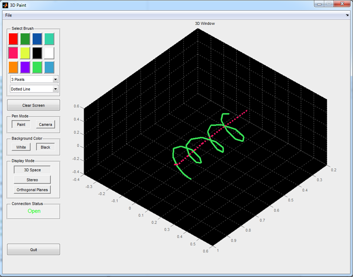
3D Paint MATLAB GUI
MATLAB initialized by setting up the serial object to talk with the 644, creating various global variables that are passed around the GUI (like brush color), and configuring various particulars about the GUI (like plot color and axis size). It also created a very important timer object. The timer object worked almost exactly like a 644 timer would. We set up how often we wanted it to execute (every 50 msec in our case) among other parameters and then programed a callback function for it. The vast majority of our code resided within this timer callback function. Trying to run the callback function faster than it took to execute caused the program to lock up, so we had to explore the timing of this function a bit to get it executing at maximum speed.
The first thing the callback did is send a ‘y’ to the 644 letting it know that it wanted data and then waited to receive the data. When we got the packet, we unpacked it by assigning the three delays and button state to variables used within MATLAB. It took us a fair amount of lab time to get the packet formatted just right so that MATLAB could parse it correctly. We found that comma delimiting the variables and using %d to format all incoming data worked well.

Data packet structure
Additionally, surrounding the code by try/catch statements caught any erratic packets that we didn’t want to process. When we read in the cycle delays, we also scaled them by a parameter called SLEW_OFFSET. We noticed that the instrumentation amplifiers had a slew that was quite quick even when applying massive gain, yet the slew would still cause a noticeable offset in the cycle delay times because the interrupt wasn’t triggered precisely when the pulse was received. Fortunately, the delay was generally constant so we could correct for it. The best way to calibrate this value was to observe the data streams of x, y, and z data points vs. time and adjust the value until all streams were perfectly isolated from one another when the pen was moved in only one dimension. For instance, if the value was not properly set, and you only moved the pen up and down, you would see some coupling between the z value and the x and y values. The other parameter that we fine-tuned for this was the distance between each pair of receivers. We initially measured this to get a ballpark idea, but fine-tuning it yielded much better results.
Next, if the packet was good, MATLAB would process the data from cycle delays into distance in meters. If the program was in paint mode it would buffer the distance into a buffer specifically for paint mode. Because MATLAB pulled values from the 644 at a rate not equal to the rate that they were produced on the 644, breaks in the data were reintroduced. To mitigate this we introduced a very small sliding window mean filter exactly like the one on the 644. In the case of paint mode the window was of length 3 to not detract from responsiveness too much. Each delay stream had its own mean filter. Next the filter delays were trilaterated into xyz-coordinates via the above equations and a linear interpolation between a point and its predecessor was produced.
One critical feature of the MATLAB program was to display a cursor of the current pen position on all the plots. This was necessary because otherwise the artist would have no idea where the pen was relative to the rest of the drawing before making a new stroke. Digging around online, we found a bit of undocumented MATLAB code that provided this functionality. All we needed to do was update a cursor object’s position value with the new xyz data. The cursor objects worked for both 3D and 2D plots. Thus, at this point in the timer function execution MATLAB updated all the cursor values. Note however that cursors were not implemented for any of the stereo plots, as they are not intended to be used as feedback while drawing. Instead, they were just neat things to look at after you’d drawn something, and having the cursor in the picture mildly throws off the 3D effect. Next, if the button associated with a given packet was pressed, all the plots were updated with the new data point.
If instead the program was in camera mode, then the incoming distance measurements were placed in a separate mean filtering buffer. The reason for separate buffers was that the camera mode could afford a bit more delay but had to be much more stable compared to the draw mode. In camera mode slight variations introduced by the artist's hand jiggling had to be smoothed out so that looking around the drawing was very fluid. Further, in draw mode we tried to limit feedback delay, but in camera mode this requirement wasn’t as tight, so we could mean more values (we’re using 10 currently for camera mode) and accept a slightly longer delay for the smoother camera positioning. In camera mode the xyz-coordinates were simply used to specify the location of the camera (the camera always points at the central point in the design space). Further, for the stereo plots we positioned the camera for the left and right eye according to a nice formula that Bruce Land generously provided.
Each of the toggle buttons and drop down menus on the GUI had a corresponding call back function. In each callback function, the appropriate global variable was set by whatever the artist selected for use elsewhere in the program. This was excepted only by the Display Mode toggle button, which turns on and off the visibility of the respective axes objects on top of updating a global variable.
The exit button functioned by simply deleting and deallocating any necessary objects for proper termination of the GUI. The clear button functioned by clearing all axes objects.
On the whole the MATLAB code was relatively straightforward to implement. The GUI overhead provided some interesting insight into MATLAB programming, and abusive use of the online documentation was critical to producing working code. There were many cumbersome and strange oddities of the MATLAB GUI that had to be worked out, but all said it worked well. The biggest upside to using MATLAB was the extensive infrastructure it already housed for producing things like 3D plots, exporting images, rotating plots, etc. The biggest downside was that this same extensive overhead was not designed for fast real time use. It didn't run quite as efficiently as we had liked, and further iterations of this design would almost certainly rebuild the PC program in a more flexible language for real time applications like Java.
Code Used
| Author | Description |
|---|---|
| Bruce Land | Push button debouncer |
| Bruce Land | Stereo camera position calculation |
| Moshe Lindner | Function to translate xyz-coordinate data into 2D red-blue data for anaglyphic stereo |
File Breakdown
| Name | Description |
|---|---|
| paint.c | ATmega644 paint code implementation |
| uart.c | ATmega644 code for uart, configured for baud at 38500 |
| uart.h | ATmega644 header for uart, configured for baud at 38500 |
| frontend.fig | MATLAB GUI figure |
| frontend.m | MATLAB code to support GUI |
Hardware Design & Implementation top
Hardware Overview
The hardware for this project provided very simple functionality. Again, our design philosophy compelled us to minimize the footprint and complexity of hardware to both keep the physical manifestation simple and to interfere as little as possible with the artist’s workflow. We designed and implemented compact, efficient analog circuitry and supporting stands to optimize portability, footprint, and quality.
The Stand and Pen
The stand was implemented out of thin rectangular wood totaling 1 inch on a side. It featured a center joint made of a screw and nut about which the stand could fold so that the device could be easily moved about. Originally, the stand was constructed with three arms, one for each orthogonal axis, with holes drilled at the end of each axis to mount a receiver. John Russell, a fellow Cornellian, thought up the center joint folding mechanism. Pictured below is a schematic view of what the original design looked like.
Initial stand implementation
This design had one advantage over the final design, being that the extra arm inherently stabilized the stand (although this was accounted for in the final design with an extra supporting beam). There were two fundamental drawbacks, however. First, due to the nature of the sphere equations generated with such receiver placement, trilateration was much more complex. While it was still possible to calculate xyz-coordinate values, the equations were sufficiently complex to possibly slow down the throughput of the system. Secondly, and most detrimentally, was that in this design we had not considered the directionality of the receivers and transmitters. A quick look at the ultrasonic datasheet showed that they had a -6 dB width of around 60°, which was wonderfully spread but still insufficient with the original design. There were very few ways you could position the pen such that all three receivers would be triggered by a single pulse. We tried moving the receivers in closer to the origin (they were originally positioned about ¾ of a meter out and we moved them to roughly .3 m out) and found nominal gains but the system still did not function as designed. The pen was simply not operational over a large enough design space.
We consulted Karl Gluck and David DeTomaso’s final project and found their solution: mount all three receivers in one plane facing the design space so that the pen could always be pointed normal to that plane. This along with the fairly wide directionality of the Rx/Tx pairs allowed a single Tx to maintain constant connectivity with all three Rx’s simultaneously. Gluck and DeTomaso’s documentation provided a shortcut to a great design that might have taken us more time to converge on otherwise.
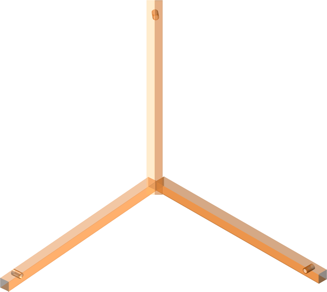
The final implementation can be seen below. Note that the stand featured a supporting arm for stabilization. We drilled a number of different receiver placement positions because the wider they were placed the greater sensitivity the device would have, yet they could not be too spread or else directionality issues would again become relevant. We converged on a happy medium by moving each receiver 47.00 cm from the origin.

2D schematic of the final stand

3D schematic of the final stand
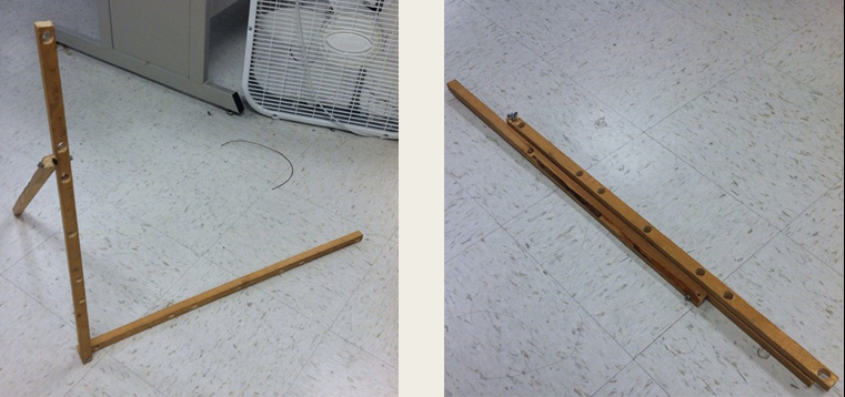
The deployed stand (left) and folded stand (right)
The pen was constructed from an emergency whistle. We drilled a hole on top to mount a single pull single throw push button and another hole on the front to mount the ultrasonic transmitter. The button's circuity was very simple as elucidated by the following schematic.

Pen button schematic
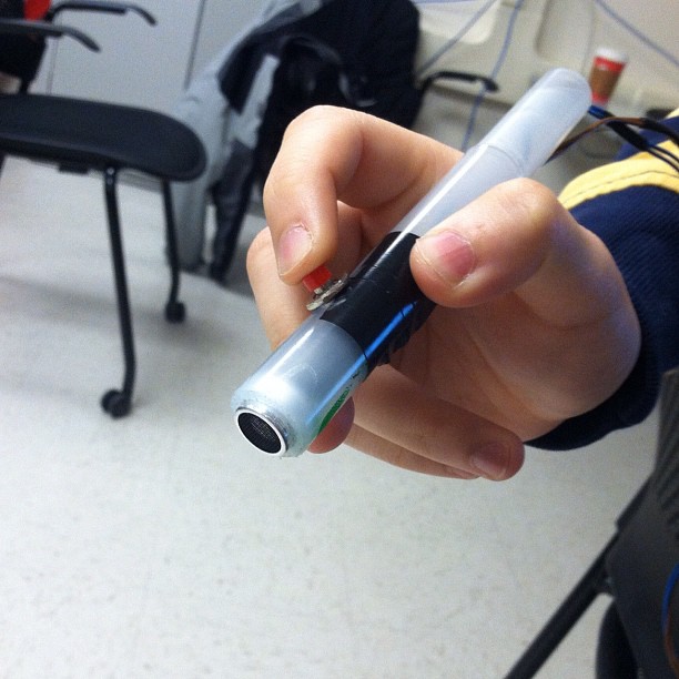
Pen
Analog Circuitry
Transmitter Drivers
We bought two ultrasonic Rx/Tx pairs from Jameco with the intention of using one of the transmitters as a receiver. We should have bought more than the minimum number required for the project. They were sharply resonant at 40 kHz, which was appropriate for use with the ATmega644, which could easily generate the necessary signal to drive them. They had a -6 dB point for a beam angle of 60° which was sufficiently spread for the project. Further, they had a fairly constant response over a wide range of operation temperatures (30°C-80°C). Also, they were designed to handle 30 V RMS driving voltage, so we could drive a very strong acoustic pressure wave from them.
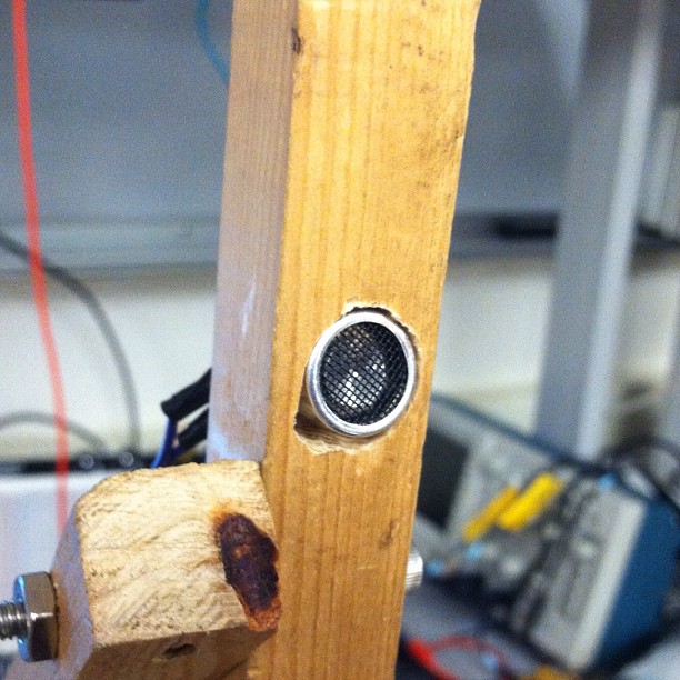
An ultrasonic receiver mounted in the supporting stand
Unfortunately, the construction of the Rx/Tx pairs was not particularly thorough. To our horror, one of the pins became loose as we were trying to wrap up the project. This obviously implied a larger problem internally, as whatever the pin was soldered to had almost certainly been severed away. We attempted to perform emergency surgery on the device to no avail, in part because the wire that the pin had been soldered to was so precariously small. Bruce Land was able to find some spare ultrasonic Tx/Rx’s in the lab, and astoundingly they were also resonant at 40 kHz. Unfortunately, they were much more directional than the Jameco equivalents. And, while we were able to produce quality results with the replacement part, it limited our design space too greatly. Admitting defeat we promptly ordered 3 spare Rx/Tx pairs. Implementing these produced the encouraging results reported later on this page.
As previously alluded to, we needed to drive the ultrasonic transmitter with a very powerful signal to produce the strongest response possible on the receive side. While an op-amp would probably be sufficient, we found that MOSFET drivers provided a very simple and effective design and thus chose a Microchip TC4428. Such an implementation was originally seen done by of Craig craigsarea.com. Because we were gaining a square wave, and because the microcontroller 40 kHz output (0-5 V) was perfectly suited for logic lows and highs a single driver chip with both inverting and non-inverting internal drivers was used. The non-inverting driver would output Vcc if it saw a voltage greater than .8 V on the input and ground otherwise. The inverting driver swapped this mapping. The following oscilloscope capture shows both the microcontroller output (channel 1) and the gained output (channel 2).
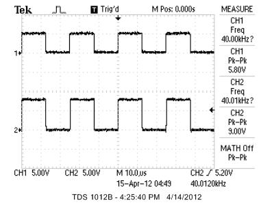
Channel 1: Microcontroller output; Channel 2: MOSFET output
Setting Vcc to 9 V (so that the device could be operated using a 9 V battery) and running our 40 kHz output from the 644 to both the inverting and non-inverting inputs, we could generate an 18 V swing from a single power source, because the inverting and non inverting outputs would each produce a 9 V swing perfectly out of phase. The following oscilloscope capture shows the inverting (channel 1) and non-inverting (channel 2) output.
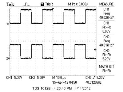
Channel 1: Inverting output; Channel 2: Non-inverting output
Hooking up these outputs to either pin on the ultrasonic Tx produced a sufficiently strong acoustic signal according to the following schematic.

Transmitter driver circuit
Receiver Circuitry
Receiver circuits are generally implemented with a cascaded series of op-amps that perform gain and band limiting filtering. Going into this project, we had no idea what kind of voltages our receiver would produce, and thus setting the gain on our receiver circuit was a guessing game. One of the suggestions Gluck and DeTomaso had in their final write up was that they would have gained the signal using a single instrumentation amplifier followed by a high-speed op-amp. Heeding this advice, we found that the Texas Instruments INA129 iamp was ideal due to its larger operating voltage (+/- 18 V) and fast slew rate 4 V/μs. A high slew rate was essential so that the iamp could properly gain the quickly oscillating 40 kHz signal and minimize the time delay between received pulse and triggering of the microcontroller. The INA129 checks in at around $7 a chip, and because we needed 3 of them we looked for ways to sample. TI graciously provided us 8 samples. Because the 1NA129 could produce 10,000 gain in one stage, we did not require the use of a subsequent op-amp for further gain
One of the nicest things about the iamp was that it accepted a differential input (perfect for the ultrasonic receiver) and only required a single resistor to set the gain. We chose a gain of 4941 by using a resistor of 10Ω via the following equation:
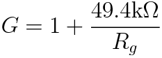
INA129 gain equation
The output of the iamp was wired up to a respective pin on the microcontroller. This gain gave our received signal a peak to peak swing around 6 V, ideal for triggering external interrupts on the 644. We additionally used Vcc = 9 V and provided some capacitors to ground to stabilize operation. This was the easiest gain implementation we’ve ever come across. We highly recommend the use of the INA129 for any and all gain applications with loose budgetary constraints and humbly thank TI for allowing us to sample them. The following schematic diagrams the external and internal operation of the INA129 receiver circuitry.
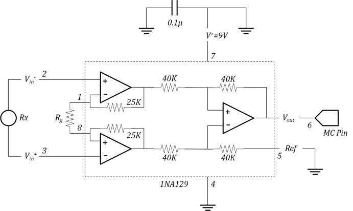
INA129 receiver circuit
We implemented all of this initially on a whiteboard. Moving over to a soldered implementation, we made all the circuitry take up only about 3 square inches. The following pictures show the final soldered circuitry and a pin diagram for how to properly wire everything up.

Pin diagram
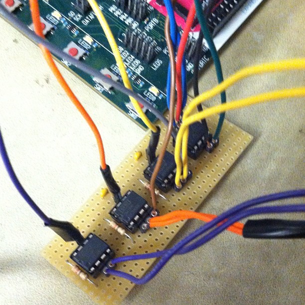
Soldered circuit implementation
Results top
Delay Accuracy & Stability
The device operated very well within a reasonable design space. We limited the axes length (and thus implied operational range) to roughly 1 meter. Within this region, our raw data was fairly accurate, so post filtering we saw very good results. The following plot shows the pen held at a constant distance from a single receiver. The raw data points are plotted along with a filtered curve.
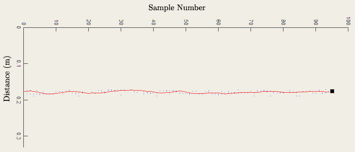
Single receiver accuracy
For this test we held the pen at 17.42 m from the transmitter, and MATLAB reported a mean filtered distance of 17.45 m, which was an acceptable error for our purposes. As witnessed from the plot, the data deviated very little from this average.
When we tested all receivers at once, we ensured that their delay streams accurately represented how the pen moved and that they all remained stable while the pen was stationary. The following diagram shows actual data while the pen was moving and while the pen was stationary.
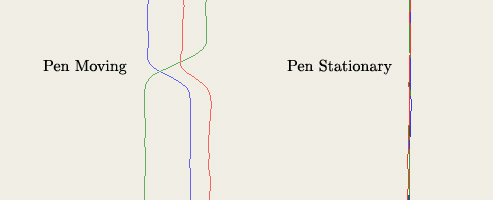
Multi-receiver accuracy
Isolation
The hallmark test for proper functionality was watching how our trilateration equations interpreted pen movements in real time. Initially we faced a large amount of coupling between the x, y, and z coordinates, with each coordinate unexpectedly following when another was varied. We corrected for this by manually calibrating two variables in the MATLAB code for optimal results. The first, as previously mentioned, was the variable SLEW_OFFSET, which allowed us to effectively reduce coupling between the different coordinates. The second was the length variable, which set the variable l used in our trilateration equations.
The following images portray the quality of isolation we managed to achieve. For each panel, the pen was displaced in a different orthogonal direction. Hence, in each graph, two of the three lines should have ideally remained completely flat, while the third, representing the coordinates in the direction of motion, should have varied in a sinusoidal pattern. In these graphs, blue represents the x coordinates, green represents the y coordinates, and red represents the z coordinates.
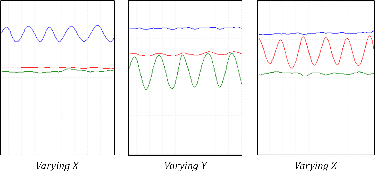
Coordinate isolation
3D Accuracy
Ultimately, 3D Paint was able to fairly accurately represent the motion of the artist’s pen. We tested the accuracy of the device by attempting to draw a perfect right angle in the yz-plane. We held a rectangular box and used the pen to trace out one of its corners, trying our best to maintain a fixed distance between the pen and the frame. This resulted in the images below, with a nearly perfect right angle seen in the yz-plane, and flat lines seen in the xy and xz-planes.
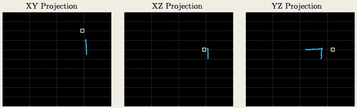
Right angle accuracy
Different Display Modes
The following GUI exports represent the functionality of the device as a whole. We will use the same drawing, a helix with a line through the middle, throughout this discussion so that the reader can see how each plot represents the same data differently.
First is the 3D projection of the helix. In this mode, as previously iterated, the artist can navigate around the helix by switching into camera mode and moving the drawing pen.
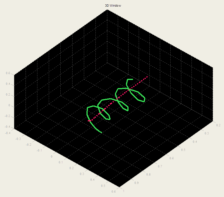
'3D Space' helix
Next are the three orthogonal projections of the data onto the xy, yz, and xz planes. We found this to be the best mode to draw in because lining up the pen and thinking in 2D was much simpler.
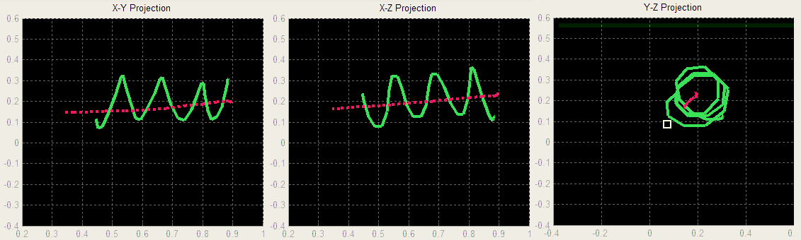
'Orthogonal Planes' helix
The following two images depict the stereo representations of the data. First is the stereoscopic representation, which is simply the same 3D data plotted from slightly separated angles to simulate viewing a real object with two eyes. By getting very close and crossing your eyes much like a Magic Eye (or by using special stereoscopic goggles) the image can be seen to pop out of the screen. This stereo plot will also rotate with camera position.
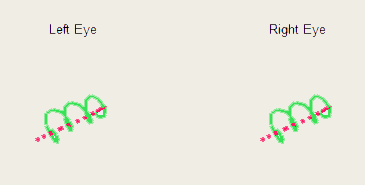
'Stereoscopic' helix
Finally we have the anaglyphic representation. This plot does not rotate with camera angle, and displays the image in a 2D plot with red/blue representations (slight depth offsets) overlaid.
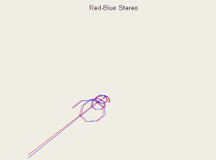
'Anaglyphic' helix
Speed of Execution
3D Paint is currently able to execute with a 0.5 second time lag between the artist moving the pen and the stroke being portrayed in the MATLAB GUI. The image below portrays this time lag. Here, the artist moves the pen at 4.0 seconds (gridline). However, the curve does not change direction until around 4.5 seconds.
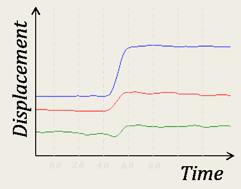
Response time
The main bottleneck occurs in the MATLAB code, as MATLAB is not well suited to operating in real time. As previously mentioned, shifting some of the signal processing onto the ATmega644 helped improve the speed incrementally.
Enforcing Safety
As with any other electronic device, operating 3D Paint has its inherent safety issues. Fortunately though, our device avoids the pesky dangers related to radio frequency or electromagnetic transmission. Hence, we focused on the usual issues of electrical insulation and grounding. While constructing the hardware, we ensured minimal strain on wires and pins to prevent unanticipated electrical shorts. Preferably, the current design should only be wired up by either of us, as we are familiar with the circuits. If hooked up incorrectly some of the ICs (particularly the MOSFET driver) may generate high amounts of heat.
Interference with Other Designs
Throughout the design, building, and testing process, we did not encounter any form of interference with other people's designs and devices. One possible source of interference, though, would be if another device made use of ultrasonic sensing of the same frequency. Under certain circumstances, it would become impossible for the receivers to distinguish where exactly the ultrasonic wave came from. In the case of our device, such interference would make it impossible to decipher the coordinates of the pen. However, due to the limited range and directionality of our ultrasonic transmitters and receivers, such undesired interference is unlikely if conflicting devices are well isolated.
Usability
We designed 3D Paint to be used by people of all age groups and from all walks of life. There are no hazardous components, and short of ripping the circuit apart, few possibilities for injury to the artist. Operation of the device literally only requires the artist to press a button on the pen and select a few options from a MATLAB GUI. As such, we believe that, like everyone else, individuals with mental or physical disabilities will be able to enjoy the visual beauty of the device's output. There are also no parts that small children might choke on.
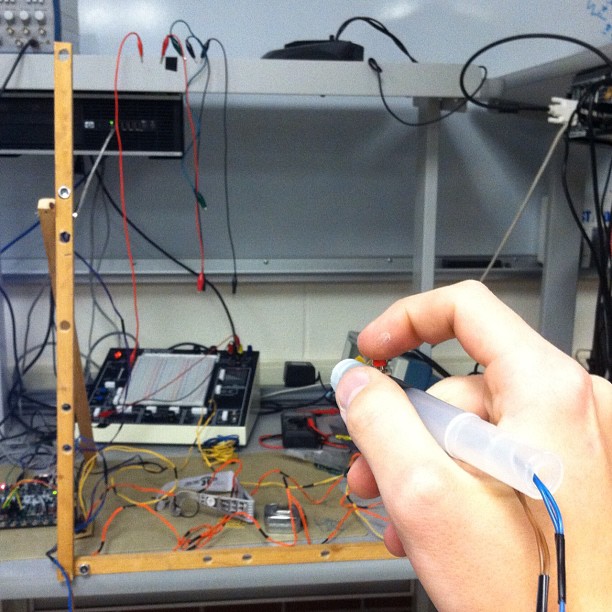
The artist's point of view
Conclusions top
Final Thoughts
We were quite satisfied with how our implementation turned out. During final testing and calibration, we felt that in fact, the system worked well enough to expose our poor artistic skills, which represented the true bottleneck in terms of quality of images produced. Using supports to direct the pen, we found that highly accurate information was captured and displayed by the system.
We would sincerely like to see what a genuine artist could do with such a device. We say this not only because we are interested in seeing how finely the system can interpret someone with artistic mastery, but also because we are curious as to how they will exploit a 3D canvas for different types of drawings.
Project Benchmarks
These are our initial objectives listed in order of when they were implemented. These requirements were outlined in our project proposal.
| Objective (The artist may...) | Achieved? |
|---|---|
| Select certain standard view angles (x-y plane, x-z plane, etc.) | Yes |
| Paint one point at a time with iterative clicks of a push button | Yes |
| Paint continuous curves by holding down the push button | Yes |
| Select different paint colors to be drawn on the MATLAB screen | Yes |
| Toggle between paint and camera modes | Yes |
| Look around the painted object my moving the pen in camera mode | Yes |
| View the painted object in stereo mode (3D) | Yes |
| Output their drawing as a picture via the MATLAB Program | Yes |
We additionally implemented the following features: anaglyphic stereo display, background color selection, clear screen, and different brush types and sizes.
Iteration Suggestions
Our finished product met most of our performance expectations. There are, however, a few areas in which we could have improved the efficiency of our design process. Firstly, we could have tested the operation of the components more extensively before soldering devices or constructing the wooden frame. As a team, we had simultaneously soldered components onto a perfboard, constructed a wooden frame, and developed the microcontroller and MATLAB code. When we attempted to integrate these different components, we faced numerous errors, and debugging became immensely tedious as it was hard to decipher where these errors originated from. In addition, after detecting the errors, we had to make inconvenient modifications to the physical circuit and wooden structure. For instance, the entire wooden frame had to be remodeled so that the ultrasonic receivers were all faced in one direction. Also, multiple holes had to be drilled at different stages to improve directionality. Next time, we will use a whiteboard and mount the ultrasonic transducers on a makeshift frame before assembling the physical components.
In addition, we broke one of the ultrasonic receivers during testing. This was an immensely costly problem as we then had to order spare parts and pay for rush delivery. This not only created a financial burden, but delayed the progress of our project.
In terms of improving our current design, we would like to mount the ultrasonic sensors on a computer monitor instead of a wooden frame in order to make the device less obstructive and more convenient to the artist as demonstrated by Gluck and DeTomaso. In addition, the oscillator could be implemented on the pen instead of being driven from the microcontroller unit. This, together with Bluetooth communication, would allow us to make the device completely wireless, thus enhancing artist freedom and mobility.
An accelerometer could also be installed on the pen to gauge when the pen is moving. Hence, we could set the pen such that it only “paints” (i.e. sends data) when motion is detected. Finally, if give more time, we would not use MATLAB to process information and instead generate a graphical artist interface in a more flexible language. By its construction, MATLAB is not suited for real time operation. This resulted in a noticeable time lag in the operation of our current device.
Conforming to the Applicable Standards
Our design adhered strictly to the aforementioned RS232 communication standard. Given the relatively simple design of our hardware, we did not find a need to modify how data was transmitted.
Intellectual Property Considerations
To our knowledge, we did not reuse code from someone else's design. The microcontroller code was in some ways similar to that employed in the previous labs, while the MATLAB code makes use of standard functions, including those used to plot images. The only exception was the code used to align the stereo images for three-dimensional projection. [Reference incl. in appendix]
Our work builds largely upon earlier work in ultrasonic positioning, using a lot of the same equipment (i.e. ultrasonic transmitters and receivers) as well as concepts (i.e. trilateration equations). However, our completed design differs from previous work in various ways. In particular, we have made the incremental improvement of recording all three positional coordinates of points in space. As previously mentioned, we do not believe that we have violated any existing patents (See Relevant Patents for a detailed listing and description).
Hence, previous designs matched ours in terms of capabilities, but not applications. Our device's ability to record three-dimensional data is a landmark improvement to these previous designs. There is, however, one patent we came across that makes similar use of ultrasonic sensing to record three-dimensional coordinates. Designed by students at Worcester Polytechnic Institute, the device incorporates a small wireless transmitter and five precisely placed receivers, with one serving as a reference. Intended as a 3D mouse, the device is able to detect motion in the third dimension, which may be interpreted as a mouse click or other manipulations. Due to significant overlap in the concepts applied in our design with a combination of previous ones, we do not believe that there are any patent opportunities. The concepts and equipment we used have long been known and readily available. The aforementioned patent is the first to make use of three-dimensional coordinates in an integral fashion.
Despite the obvious similarities with the 3D mouse, we believe there may be publishing opportunities for our device. Unlike the 3D mouse, it is able to record coordinates with only three ultrasonic sensors (their design using a hefty frame with five precisely positioned sensors). These may be conveniently placed at the three corners of a computer monitor as Gluck and DeTomaso did to create a uniquely unobtrusive artist experience. This is thus a more economical and practical alternative.
We did not have to sign any non-disclosure agreements to get sample parts.
Ethical Considerations
To our knowledge, the decisions we made and actions we took on this project were consistent with the IEEE Code of Ethics (In the following paragraphs, the numbers indicated in parentheses indicate which of the 10 codes of ethics each section relates to).
In particular, we ensured that our project did not in any way infringe on the safety, health, and welfare of the community or environment (1). Before embarking on our project, we ensured that the ultrasonic transmitters we employed did not cause irritation to the people around us. In addition, we practiced the utmost caution during the fabrication process. As plastic is highly toxic in vapor form, we ensured to isolate plastic components when soldering. We also consistently checked if our device was dissipating large amounts of heat in order to avoid the possibility to causing electrical explosions. We thus took every precaution to avoid causing others physical harm (9).
Throughout the process of reporting our findings, we have also maintained objectivity and have not conspired to making sweeping claims (3). We acknowledge that though we have made significant improvements on previous designs, our finished product does not by any means represent a paradigm shift.
In addition, through creating a detailed write up of the concepts and technologies employed, we feel that we have done our utmost to improve the understanding of existing technologies and their applications as well as consequences (5). We believe that we have helped to elucidate the potential and shortcomings of ultrasonic sensing technology.
We have also made every attempt to acknowledge the previous findings of others. If our work is adapted and referenced in the future, we will be open and accepting of criticism (7).
In line with the code of ethics, when working on our project we made every attempt to assist our classmates in their professional development (10). For instance, we were able to guide another group by helping them export data from their MCU to MATLAB in real time.
We also restricted ourselves to only making use of technologies and techniques that our education has trained us to employ (6). AVR Studio and MATLAB are programs that we have developed mastery of through previous projects. In addition, the classes we have taken as Electrical and Computer Engineering undergraduates have given us a plethora of experiences soldering both through hole and surface mount devices.
Finally, we also made sure to treat all our peers fairly regardless of race, religion, gender, disability, age, or national origin (8). In fact, the two of us are of different race and national origins, and have maintained a fair and equal working relationship over the past semester.
There were few, if any avenues for conflicts of interest (2) or bribery (4) throughout this project.
Legal Considerations
Our project makes use of a single ultrasonic transmitter operating at 40 kHz (far beyond the human audible range of 20 Hz to 20 kHz). As such, we do not make use of any electromagnetic wave transmitters, and the operation of our device is not regulated by the Federal Communications Commission (FCC).
One caveat, however, is that the ultrasonic wave emitted by our transmitter is well within the hearing range of some pets (cats and dogs: 40 Hz to 60 kHz) and pests (mice: 1 kHz to 70 kHz). Hence, operation of our device in a household setting may cause significant irritation to pets, as well as causing pest related issues. Before the device is commercially deployed, research must be undertaken to ensure that the noise produced be at acceptably low amplitudes to avoid animal irritation and hearing damage
In addition, we have taken every precaution to make the device safe for the everyday artist, including but not limited to checking for shorts and the insulation of wires, and ensuring the grounding of relevant surfaces.
Appendices top
A. Parts List and Costs
S: Sampled, P: Purchased, F: Found
| Category | Item | Type | Vendor | Unit Cost | Quantity | Total Cost |
|---|---|---|---|---|---|---|
| Electronics | STK 500 | P | ECE 4760 Lab | $15.00 | 1 | $15.00 |
| Mega644 | P | ECE 4760 Lab | $6.00 | 1 | $6.00 | |
| 9V Power Supply | P | ECE 4760 Lab | $5.00 | 1 | $5.00 | |
| Ultrasonic Tx/Rx Pair (Jameco Valuepro 40T/R-12B) | P | Jameco (Part No.: 139492) | $7.95 | 2 | $15.90 | |
| 1.5A Dual Mosfet Driver (Microchip TC4428AEPA) | P | Jameco (Part No.: 1292826) | $1.09 | 1 | $1.09 | |
| Instrumentation Amplifiers (Texas Instruments INA129) | S | Texas Instruments Inc. | $0.00 | 3 | $0.00 | |
| Connections | Small Solder Board (2 inch) | P | ECE 4760 Lab | $1.00 | 1 | $1.00 |
| 8 pin DIP Socket | P | ECE 4760 Lab | $0.50 | 4 | $2.00 | |
| SIP Socket | P | ECE 4760 Lab | $0.05 | 13 | $0.65 | |
| SIP Plug | P | ECE 4760 Lab | $0.05 | 3 | $0.15 | |
| Header Socket | P | ECE 4760 Lab | $0.05 | 9 | $0.45 | |
| Wire | F | ECE 4760 Lab | $0.00 | N.A. | $0.00 | |
| Button | F | ECE 4760 Lab (Scrap) | $0.00 | 1 | $0.00 | |
| Resistors and Capacitors | Through-Hole 10Ω Resistor | F | Already owned | $0.00 | 3 | $0.00 |
| Through Hole 0.1µF Capacitor | F | Already owned | $0.00 | 3 | $0.00 | |
| Physical Structures | Pen Casing | F | Already owned | $0.00 | 1 | $0.00 |
| 3 foot wooden plank | F | Already owned | $0.00 | 3 | $0.00 | |
| Screw | F | Already owned | $0.00 | 2 | $0.00 | |
| Nut | F | Already owned | $0.00 | 2 | $0.00 | |
| Washer | F | Already owned | $0.00 | 2 | $0.00 | |
| Total | $47.24 |
B. Source Code
Please email us to request the source code for either the ATmega644 or MATLAB.
C. Specific Task Breakdown
| William Myers | Both | Guo Jie Chin |
|---|---|---|
| Stand construction | Stand design | Stand refinement |
| Microcontroller code | Hardware design | Wiring, connections, and debugging |
| MATLAB code | Debugging | Website graphics |
| Website formatting | Website content |
D. Relevant Patents
| Sonic Positioning Device |
|---|
| Inventor: Ronald E. Milner |
| Patent number: 4862152 |
| Filing date: Jan 25, 1985, Issue date: Aug 29, 1989 |
| Abstract: A three-dimensional ultrasonic position control device suitable for controlling computer displays or robot movements is disclosed. |
| Notes: This early work uses similar equations for triangulation. However, it only measures a point's coordinates in a two-dimensional plane, without attempting to interpret the position of points in three-dimensions. |
| Ultrasonic wireless pen position determination system and method |
|---|
| Inventor: Jianping Xu |
| Patent number: 6535206 |
| Filing date: Feb 18, 2000, Issue date: Mar 18, 2003 |
| Abstract: The invention in one embodiment provides a system and method for determining the position of an ultrasonic pen device, and for providing calculated position information to a computer system. The system of one embodiment comprises a first and second ultrasonic sensor that detect an ultrasonic signal emitted by an ultrasonic pen. The system further includes analog-to-digital converters to digitize the sensed ultrasonic signal and a processor to process the ultrasonic signal and determine the position of the ultrasonic pen. |
| Notes: This design makes use of only 2 ultrasonic receivers, and is therefore unable to derive coordinates in three-dimensions. |
| Acoustic based pointing device |
|---|
| Inventors: Miroslav Trajkovic, Antonio Colmenarez, Srinivas Gutta |
| Patent number: 7158126 |
| Filing date: Apr 8, 2002, Issue date: Jan 2, 2007 |
| Abstract: An acoustic based pointing device and a system and method for using the pointing device to move a cursor on a display screen of a display device. The pointing device comprises an acoustic source that generates and propagates an acoustic signal that is detected by four microphones M1, M2, M3, and M4 and is then converted into corresponding periodic electrical signals S1, S2, S3, and S4. The position vector P0 of the acoustic source is calculated by solving triangulation equations that depend on phase-shift time delays between S1 and Sj for j=1, 2, and 3. A position vector PC is calculated from P0 using a scale vector that relates a change in position of the cursor to a change in position of the acoustic source. Then the cursor is moved to a position PC associated with the position vector PC. |
| Notes: This patent relates to the specific application of moving a cursor on a screen, and also does not attempt to interpret positions in three-dimensions. |
| Wireless Display Systems and Stylii |
|---|
| Inventors: Jianping Xu, Stephen H. Hunt |
| Patent number: 7248251 |
| Filing date: Mar 5, 2004, Issue date: Jul 24, 2007 |
| Abstract: A wireless coordinate input system for a display system includes a stylus that transmits ultrasonic energy to a plurality of ultrasonic receiving stations in a projection plane. In an embodiment, the stylus may include one ultrasonic transmitter used for determination of three-dimensional coordinates of the stylus relative to the projection plane. The stylus may also include a second ultrasonic transmitter controlled by a pressure-activated switch. When the stylus is pressed against the projection plane, the second transmitter turns on and is used for determination of two-dimensional coordinates of the stylus in the projection plane. The stylus may also include a higher frequency burst transmitter used to generate a time reference. On or more of the ultrasonic receiving stations may also include an ultrasonic sensor for calibration. |
| Notes: This patent, held by Intel Corporation, describes a design that has the capability of determining three-dimensional coordinates but similarly does not attempt to interpret positions in three-dimensions. |
| Apparatus and method for determining the position of an object in three-dimensional space |
|---|
| Inventors: Christian Banker, Michael Cretella, Jeff Dimaria, Jamie Mitchell, Jeff Tucker, Brian King |
| Patent number: 7668046 |
| Filing date: Jun 6, 2008, Issue date: Feb 23, 2010 |
| Abstract: An apparatus and method is disclosed for determining the position of a artist interface mouse using time of arrival measurements. A transmitter transmits a signal to an array of receivers that are spatially separated from one another. The time difference of arrival for is found for each receiver relative to a predetermined reference receiver. Using the time difference of arrival (TDOA) of each receiver, the location in three-dimensional space of each receiver, and the speed of sound the position of the transmitter in three-dimensional space relative to the reference receiver may be found. |
| Notes: This design is far more complicated than ours, and makes use of five ultrasonic receivers (with one set as a reference point) to determine the position of an object in three-dimensions. It was created by students at Worcester Polytechnic Institute in Massachusetts, and featured in popular science magazine. |
References top
This section provides links to external documents, code, and websites referenced and used throughout the project.
Datasheets
- Ultrasonic Tx/Rx Pair (Jameco Valuepro 40T/R-12B)
- 1.5A Dual Mosfet Driver (Microchip TC4428AEPA)
- Instrumentation Amplifiers (Texas Instruments INA129)
- ATmega644
Vendors
Background Info
References
Acknowledgements top
We are going to radically depart from the norm and extend our fullest gratitude to Bruce Land for his thorough and insightful guidance in ECE 4760. Further, we appreciate the effort all 4760 TAs put forth on our behalf, specifically our section instructors Joseph Montanino and Pavel Vasilev. Further we would like to acknowledge the Cornell ECE department and all the wonderful instructors we have had over the years.
Our gratitude goes out to Texas Instruments for providing the top-notch INA129 instrumentation amplifiers free of charge.
We thank Kevin Fuhr for continually aiding us in drilling holes for the stand and John Russell for his mechanical insight when designing the stand.