Cornell University ECE4760
DSP
Pi Pico RP2040
This page covers several DSP topics including:
IIR filters in s7x24 fixed point format at 40 KHz rate.
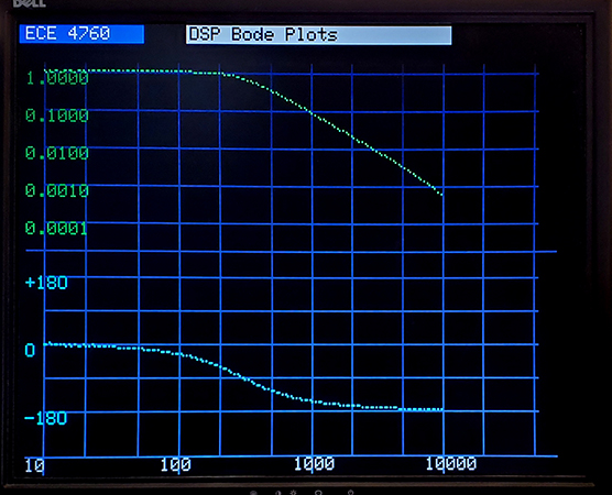
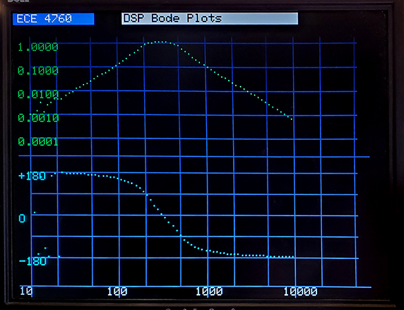
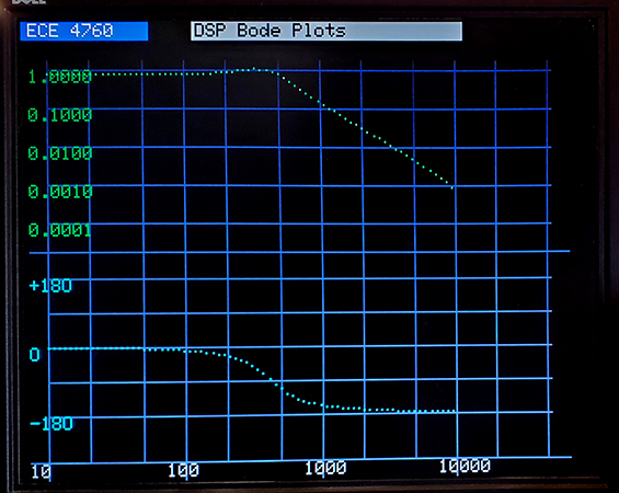
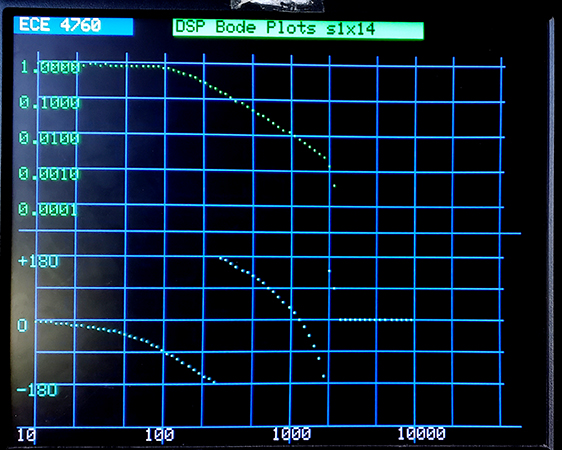
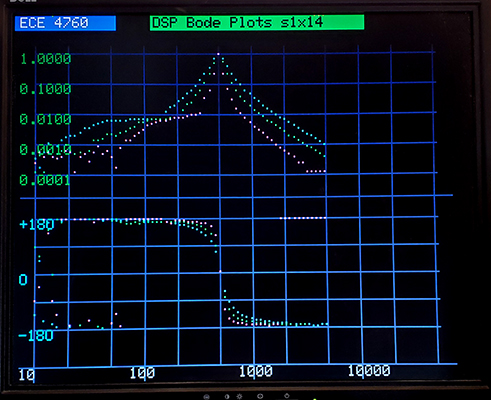
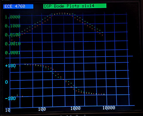
The code implements Butterworth and type-1 Chebychev low pass filters and Butterworth bandpass filters. For testing, the filter Bode plots are displayed on the VGA interface. Three plots below are:
--
2-pole lowpass Butterworth with cutoff 300 Hz;
--
4-pole bandpass Butterworth with cutoffs at 200 and 500 Hz;
--
2-pole type-1 Chebychev lowpass with cutoff 500 Hz and 3 db of passband ripple.
All filters were designed in Octave, then the constants are pasted into the filters, where they are converted to fixed point. More than 5 digits of accuracy are necessary for the 4-pole filters. The "Direct Form II Transposed" implementation of a difference equation shown below (from the Matlab or Octave filter description).
    a(1)*y(n) = b(1)*x(n) + b(2)*x(n-1) + ... + b(nb+1)*x(n-nb)
                          - a(2)*y(n-1) - ... - a(na+1)*y(n-na)
The y(n) term is the current filter output and x(n) is the current filter input. The a's and b's are constant coefficients, determined by some design process. Usually, a(1) is set to one. You can use the Matlab or Octave filter design tools to determine the a's and b's.
Frequency grid lines are logarithmic, with decade, 2's (e.g. 20,200,200) and 5's (e.g. 50, 500, 5000) drawn. Amplitude in the upper plot is logarithmic, with decade lines drawn and labeled. Phase in the lower plot is a linear scale. The 4-pole plot has some incorrect points at low frequency because the averaging time of the cross-correlation used to get the phase and magnutude did not average enough samples. To get phase and magnitude, the filter output was cross-correlated with the filter input sine wave, and a 90-degree phased shifted version of the sine wave. These are refered to as the I (in-phase) and Q (quatrature) channels of the correlation. You can think of the I and Q signals as the vector components of the output voltage. The average value of the magnitude of the vector is the output amplitide and the arctan of the ratio of the average of I and Q is the phase. The first image is a 2-pole Butterworth lowpass at 300 Hz. The second is a 4-pole Butterworth bandpass. The third is a Chebychev type-1 lowpass with a few db of bandpass ripple.
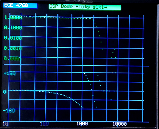
IIR filters in s1x14 fixed point format with CIC downsampler.
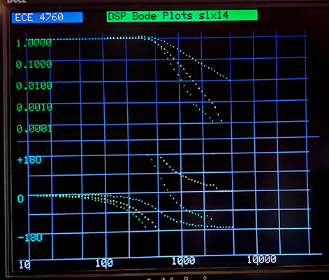
These filters are second order only. For both Chebychev type 1 filters and Butterworth filters, the filters are stable down to bandwidth/Nyquist of 0.01 or so. With the full sample rate of 40KHz (Nyquist rate 20KHz), then downsampling by 4, the Nyquist rate is 5KHz. The 4th order CIC filter, plus Chebshev compensator has a rapid cutoff at 2 KHz, or 0.4 normalized to the new Nyquist rate. The first image below is the downsampler Bode plot. Note the fast cutoff at 2KHz, dropping to below 0.001 amplitude before the 5KHz Nyquest rate. The second plot is a Butterworth 2-pole lowpass feed by the downsampler. The cutoff of the lowpass is 0.025 of the downsampled Nyquist rate.
The downsampler, and each 2-pole filter takes about 0.8 uSec to execute, at standard clock rate. The GPIO2 pin is used to time the ISR and filter sections.
IIR filters in s1x14 fixed point with downsampler, second-order-sections, and design commands.
The goals here are to implement second-order-sections and a command language to design them, without having to use tools from Python, Octave, or Matlab.
This example implements 2, 4, and 6 pole lowpass, 2 and 4 pole bandpass, and 2 pole highpass filters. The filter design is a slightly simplified version from Cookbook formulae for audio equalizer biquad filter coefficients by Robert Bristow-Johnson. There is optional down-sampling. All functions are controlled by a simple command sequence. In the commands below, the parameter Q is a measure of gain near the cutoff freqeucy, relative to the DC gain. In lowpass or high pass filters, it trades off passband flatness for faster cutoff. In bandpass filters it sets the sharpness of the filter. Some example Q values for a 2-pole lowpass:
Q       0.5       0.707        0.9        1.0   1.1     1.2  1.5  2.0
peak   droops     flat         1.05       1.1   1.2     1.3  1.5  1.9
name   RC       Butterworth  Chebyshev          Cheby
                             0.5 db ripple      2 db
The commands for building and displaying filter responses are shown below.
Some examples are shown below.
The first plot is for three bp4 filters with Q of 4 to 10(sharpest).
The second is the hp2lp2 4-pole bandpass filter with Q 0f 0.707 and cutoffs of (200,1000) and (300,700).
The third is 2, 4, and 6 pole lowpass filters all set to cutoff of 500 Hz and Qs chosen to be as flat as possible by educated guess of Qs.
The program is bulky because it handles the graphics to plot the frequency responses, supports a command language, computes the filter coeffients from user specifications, specifies several filter types, and runs a 40 KHz ISR to actually do the filtering. This ISR sweeps a frequency over the desired range using DDS, runs the desired digital filter using the DDS as input, then computes the cross-correlation of the filter output with the DDS input, and with a second DDS signal which is in quadrature with the filter input. From the average correlations, the graphics thread computes the Bode plots of filter phase and magnitude. The phase/magnitude calculations become inaccurate at very low frequency, or low filter output amplitude. You can see that in the bandpass plots above.
Spectrogram -- Audio rate
The VGA routines were used to construct an oscilloscope-like display of an ADC channel connected to a microphone. The raw waveform is displayed, plus the power spectrum, the approximate log-power spectrum, and the spectrogram. Core 0 handles the data aqusition and display. Core 1 does the FFTs and handles the serial terminal. The ADC acquires 512 samples at 16 KHz. This rate and window length is about right for speech spectrum (100-3500 Hz). The code computes the FFT bin with peak energy and displays it in the upper left corner. The serial interface starts/stops the data acqusition. The spectrogram shows about 20 seconds of 32 mSec, non-overlapped, sample windows. The code uses two interesting approximations. The first is the alpha-max, beta-min algorithm to speed up square root of sum-of-squares. It is accurate to within 6%. The second is an approximation of log base two from Generation of Products and Quotients Using Approximate Binary Logarithms for Digital Filtering Applications, IEEE Transactions on Computers 1970 vol.19 Issue No.02. It is accurate to within 0.2 log units and is represented is a weird u4x4 fixed point format. The resulting 8-bit log is accurate enough for plotting.
.jpg)
FM sound synthesis
FM synthesis is a fairly simple method of producing interesting sounds, including sounds that approximates musical instruments. The sound can be can be string-like, or drum-like, or just plain strange.
You basically have to experiment to find the sound you want. The basic waveform generation equation is:
wave = envelopemain * sin(Fmain*t + envelopefm*(sin(Ffm*t)))
For each of the amplitude envelopes, I used a simple attack, sustain, decay system, with linear amplitude increase during the attack, constant amplitude during the sustain, and linear decrease during the decay section. In the code, the FM envelope is called modulation depth because the envelope scales the size of the frequency changes. The actual sin waves are generated by direct digital synthesis DDS. All arithmetic during synthesis is carried out s19x12 fixed point. The way I scaled amplitudes required being able to represent integer values up to about 500,000. Sound is produced via a PWM channel on gpio3, with output filtered with a 2K resistor and 10nf capacitor.
The default serial output of gpio 0,1 is used.
To use the program you specify nine parameters using the serial interface:
Fout -- the main frequency in Hz.
The main waveform attack, sustain, decay (ASD) in seconds.
Fmod -- the fm modulation frequency in Hz.
The modulation depth, a float, typically in the range of 0-1.0
The modulation
attack, sustain, decay in seconds.
The progam will then repeat the sound when you hit return (twice)
The number of sounds you can make is bewildering, but a good place to start is a string-like sound by
setting Fout=220, main ASD to {0.001, 0.001, 2.0}
then Fmod=660, depth=0.25 and modulation ASD to {0.001 0.001 1.5}
FM synthesis -- with muscial scale -- better decay --
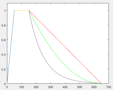
This example adds a tuned musical scale output to better evaluate the sounds. I chose to implement eight notes from C3 to C4 but in the code below, you can pick the octave. The code also adds a smoother decay function option. The linear decay is a very crude approximation (the first term of the Taylor expansion of a decaying exponential). Linear was used because its duration is finite and easy to specify, however the relatively slow decay, coupled with the sudden termination, sounds strange for some sounds.
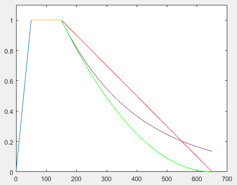
Exponential decay is easy to calculate with one multiply, but suffers from an infinite duration, so getting a clean cutoff is hard. The long, slow exponential tail also leads to some numerical accuracy problems. A quadratic decay can be arranged so that it approaches zero amplitude with zero slope and falls more rapidly than linear initially. The image shows amplitude vertically, and audio sample number horizontally. The attack phase is blue, sustain is yellow, linear decay is red, exponential decay is purple, and quadratic decay is green. Attack in this example is 50 samples, sustain is 100 and desired decay time is 500 samples.
If you adjust the exponential time constant to one-fifth of the decay cutoff, you get the first plot. The amplitude has decreased about 150 fold but the initial fall rate is fast. If you adjust the exponential time constant to match the initial slope of the quadratic, then the exponential has dropped to about 14% at the desired cutoff time, while quadratic and linear have reached zero. It is much easier to use the quadratic for a desired decay cutoff time, with a reasonalbly smooth sound near cutoff.
Actually computing the quadratic envelope requires fitting three constraints to the general quadratic form ax2+bx+c=0 to determine a, b and c. If we require that the quadratic be zero, with zero slope at the decay cutoff time, and to have the sustain amplitude when it starts, then a little algebra gives:
a = (sustain_amplitude)/(decay_time)2
b = -2*(sustain_amplitude)/(decay_time)
c =
sustain_amplitude
Since we are computing one audio sample at a time we can do a numerical integration to simplifiy the required arithmetic at each time step. Specifically, we are adding the derivitive of the quadratic to the current amplitude to perform Euler integration of the quadratic:
new_amplitude = current_amplitiude + 2*a*(fall_time) + b
Some care is needed with operation order to maintain accuracy in fixed point. When running in an ISR, the worst case timing is 3.8 uSec with quadratic decay and 2.5 uSec with linear decay.
Example scales:
The program plays eight notes, at four different
fm depths. The depth values are
{0 .25 .5 .75}*(maximum_fm_envelope_depth)
The program inputs are now:
-- An octave number from 1 to 6, e.g. choosing 2 plays C2 to C3.
-- Amplitude attack, sustain, and decay times in seconds (floating values)
-- Chose linear or quadratic decay -- enter 1 for
linear, 0 for quadratic
-- the ratio of the modulation frequency to the main frequency
-- the maximum fm envelope depth
(a float between 0 and 2)
--
fm envelope attack, sustain, and decay times in seconds (floating values)
FM synthesis with specrogram and joystick-driven menu interface
With all the parameters necessary to specify the synthesis, I decided to build a menu system for changing the ten, or so, parameters. Also, the sounds produced are so complex that it is nice to have a spectrum and spectrogram (see the top of this page) so that the systhesis can be compared to real sounds visually. Adding a cursor and joystick to Hunter's VGA driver was an interesting exercise. The joystick is a HiLetgo Game Joystick Sensor Game Controller from Amazon. It consists of two potentiometers (x and y stick position) and a push-click button attached to the stick. The button only works when the stick is centered. Reading the state of the joystick is easy, but the potentiometers are not very well calibrated, so I decided to use the position of the joystick to determine cursor x and y movement speed, as opposed to position. Also, because of noise, and for ease of control, the speed in each direction was quantized to a few speeds in each direction. In this example cursor movement is limited to the menu region of the screen.
On every pass through the main graphics thread loop, the event loop, the cursor is erased, then redrawn at the current location specifed by adding the joystick speed to the old position. Erasing means copying the saved image pixels back to the display buffer. Drawing means saving the image pixels and replacing them with the cursor color. The cursor position is then decoded into a menu item location. A single joystickclick in a menu item enables the x potentiometer to control the menu value, as determined by a couple of constants for that item. The menu-change condition is indicated by a small red dot in the menu item. Another click, or movement of the y potentiometer, cancels the menu change mode. Double-clicking the joystick freezes the GUI and allows new value input from the serial command line. The serial menu-change mode is indicated by a small green dot, and is canceled when the user hits <enter> on the keyboard.
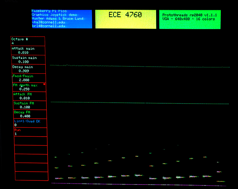
The spectrum analysis takes place at the sound synthesis rate of 40 KHz. The FFT buffer size is 2048 samples, so the FFT window size is about 50 mSec and the FFT fundamental frequency is 19.5 Hz. This resolution cannot resolve individual musical notes until about C4 (523 Hz), but seems like a good compromise between time resolution and frequency resolution.
The image below shows the FM synthesis menu, with the FM depth item highlighted for change. Top trace is the current short term spectrum, midde trace is log(spectrum) and at the bottom is the spectrogram. You can see the requency steps of the scale, with a couple of harmonics. The harmonics taper off before the fundamental because the FM envelope is shorter in duration. The fast attack time, tapering harmonics, and harmonic spacing tend to make a string-like sound.
This is a big example, so it needs an outline of the code:
There are connections to the RP2040/PICO for VGA, SPI DAC, and the joystick.
The summary is:
FM synthesis with spectrogram and rotary-encoder driven menu interface
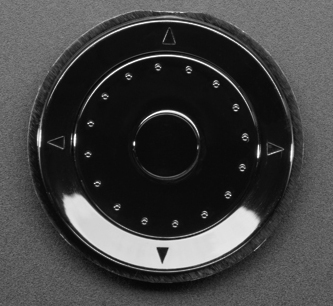
It turns out that using the joystick, above, for menu control is a little too senstive and hard to control. Using an Adafruit rotary encoder with direction arrows and a center-button is easier. In the image below, each of the four drirection pushbuttons is indicated by a small triangle near the edges. The center button is a slightly raised circle in the middle. Pushing anywhere on the circle of small dots engages the rotary encoder. Dragging clockwise and counter-clockwise changes the value of a counter. To run the FM synthesis menu, the up/down buttons change the item to be selected, and the center-button selects/deselects an item. When selected, the value of an item can be changed by scrolling the encoder. Pushing the center-button again deselects the item. Double-clicking the center button freezes the GUI and shifts value entry to the serial interface. Serial entry returns control the the GUI when you hit the <enter> key. All other functionality of the above example is the same. There is one more thread running on core0 compared to the previous code which watches for an edge on the decoder switches and determines rotation. And, of course, the joystick is disconnected and replaced with encoder connections to seven gpio ports, plus two ground connections. The Adafruit breakout board connections are on the left of the list, the PICO connections on the right.
Copyright Cornell University May 24, 2023