Cornell University ECE4760
Lattice-Boltzmann with 320x240 VGA 16-color
Pi Pico RP2040
Lattice_Boltzmann on RP2040
Lattice Boltzmann(LB) methods can be used to approximate fluid flow on a grid of cells.The algorithm approximates the equlibrium distribution of particle velocities in eight directions for each grid point, then propagates the distributions to neighboring cells. Daniel V. Schroeder at Weber State University has written a good explaination of LB, as well a very nice interactive javascript simulation. We ported the javascript to C then optimized it for the RP2040. The alogrithm is a memory hog, requiring about twelve arrays of dimension equal to the total number of grid cells. The initial, floating point, version from the javascript ran very slowly, with a time step update of 250 mSec.
Optomization:
- The first step is to convert to fixed point for speed. We chose s1x25 format (sign bit, one bit to the left of the radix point, 25 fractional bits) because it ports well to the FPGA we are using in another class. ECE5760 LB page.
- The next optimization step was to eliminate two divides per grid cell per time step by Taylor-expanding the reciprocal of the denominator and multiplying. Three terms of the expansion were kept because the fluid density (denominator) was within a few percent of unity. The approximation is shown below, with mFix being the fixed point multiply. The divide is thus converted into four adds and a multiply.
Fix rho_inv = 1 - (rho - 1) + mFix(rho - 1),(rho - 1))
- The next step was to parallelize across the two ARM cores using Protothreads primitives for syncing the calculations. The heavy computational step is the equlibrium distribution calculation which conveniently uses only information already in each individual cell. This was easy to split into left/right halfs for the two cores. The streaming step in which the fluid velocities are propagated separates into seven distinct memory copies, also easy to split.
- Drawing the fluid flow required calculating the speed of the flow from the x and y velocity components. To avoid a square-root calculation we used the simplest possible alpha-max beta-min algorithm to compute the magnitude, with alpha=1 and beta=0.5.
speed = max(abs(ux[i]), abs(uy[i])) + (min(abs(ux[i]), abs(uy[i])) >>1)
This speed approximation is good to about 8%.
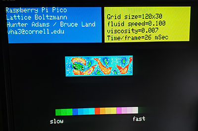
There are only 16 colors in the 4-bit VGA we used and those colors were assigned equal speed intervals for plotting.
- The screen resolution had to be reduced to 320x240 to free up RAM for the ten large arrays. This makes the text blocky, but the LB flow looks good.
The five optimization steps gave a factor of ten speed-up to about 40 updates/sec, including drawing to the screen. This is fast enough for animation of the flow.
Examples:
- LB on 120x30 region with a flat barrier to form a von Karman vortex street

Video
Project ZIP file.
C code
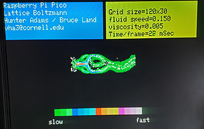
- Particle tracing (advection) in the flow was accomplished by numerically integrating the local velocity.
The tracer particle x,y coordinate integer parts give the LB cell to be interogated for the macroscopic velocity (ux, uy).
The macroscopic velocity is then vector-added to the fixed point position.
Fixed point s17x14 format was used because the pixel positions can be large.
Two examples below show tracers in the vortex street as before, and a jet hitting a barrier.
The jet is a few pixels wide and directed to the right where it hits a barrier and is deflected along two paths.
Click images for video.
Project ZIP file
Jet C code
Vortex street C code
Copyright Cornell University
April 26, 2022