Cornell University ECE4760
Laplace's equation solver
Pi Pico RP2350

Laplace's equation and Poisson's equation
Poisson's equation shows up in various physical systems, like heat flow, electorstatic voltage, and fluid flow. It describes each of these systems in the steady-state limit, so the form shown below has no time dependencies. u is some potential and f is a source term, both of which are functions of two dimensions. If f(x,y)=0, then we get Laplace's equaiton
∇²u(x,y) = f(x,y)
Numerical solution requires that the partial differential equation be converted to a discrete form, then solved using an iterative scheme. The scheme we will use is successive over-relaxation (SOR) on a 2D grid with 4 nearest neighbors. The central observation is that the value of u at any grid point is the mean of the 4 neighbors. Ths is, of course, subject to constraints, for example boundary conditions. SOR simply interates across the entire array, while updating a new point to the average of the four surrounding points, and using new values for the surounding points as soon as possible. The specific formula for update u(i,j) is shown below. This assumes that the update sweep is from low-to-high index so that the time step n+1 values of u(i-1,j) and u(i,j-1) values are known.

$u_{\mathrm{i,j}}^{\mathrm{n+1}}$ = 0.25 * Ω * ( $u_{\mathrm{i-1,j}}^{\mathrm{n+1}}$ + $u_{\mathrm{i,j-1}}^{\mathrm{n+1}}$ + $u_{\mathrm{i+1,j}}^{\mathrm{n}}$ + $u_{\mathrm{i,j+1}}^{\mathrm{n}}$ + $f_{\mathrm{i,j}}$ ) + ( 1 - Ω) * $u_{\mathrm{i,j}}^{\mathrm{n}}$

The over-relaxtion part of this refers to over-correction for faster convergence. Omega is an optimized value dependent on grid size and boundary conditioos, but has values 1.0<omega<2.0. A too small omega leads to slow convergence. Too big is unstable. You may need to experiment to find the best omega.

A further optimization for parallelization across the two cores is refered to as red/black ordering, like a checker board. During each update interation, red cells depend only of black cells and vice-versa. This allows the advantages of SOR, with minimal memory collisions between cores.

The Poisson program.
The program starts three threads. Some care is necessary to make sure the threads start in the correct order. Core 1 has only a SOR compute thread and must start first, so there are three short delays in main and in the core 0 compute thread to ensure this. The two compute threaads are controlled by a serial interface described below.

The core 0 compute thread sets up the boundary conditions and internal special conditions by making certian grid points isopotentials, insulators, or sources. The boundarys can be Neumann condition, with zero normal gradient corresponding to an insulator, or the boundarys can be Dirichlet condition with a single fixed potential. Internal insulators enforce zero nornal gradient. Internal isopoentials enforce constant potential. Internal sources act like current sources anywhere in the grid. The sum of all source strengths must be zero.

Once the initial conditions are set up, the core 0 compute thread drops into an infinite while loop where it checks for a restart thread condition, checks for continuing iterations, then signals core 1 to start a interation, then starts its part of the iteration. When core 0 finishes its part, it waits for a signal that core 1 has finished, then prints interation statistics (time, error, count). The loop just keeps running until the serial thread signals a change of some kind. Note that the iterations do not represent time evolution, but only the convergence to steady state.

The serial thread set up a serial prompt then waits for the human to type something.
Each command is terminated with the <enter> key .
A parser recognizes one of five commands. I used these mostly for testing:

• r -- forces a core 0 compute thread restart.
• c -- signals the core 0 compute thread to continue
• field -- computes and displays the gradient vector field of the potential and stops the core 0 compute thread.
  Note that the displayed vectors give direction, but only relative amplitude.
• omega value -- sets the over-relaxation parameter to 1.0<=value<2.0 and restarts the core 0 compute thread.
• bound neumann -- sets zero gradient boundary and restarts the core 0 compute thread.
• bound dirichlet value -- sets 0<=value<15 isopotential boundary and restarts the core 0 compute thread.

Internal isopotentials, insulators, and sources need to be specified in the code, as described below
The state of the grid solution is held in three arrays:

• The array u(i,j) holds the floating point current estimate of the potential.
  --The scaling is most-negative u(i,j)=0,
  -- Most-positive is u(i,j)=15.
  -- The potentials map directlly to the 16-color palatte. (potentials in the range [0,15])
• The array s(i,j) indicates the type of grid node.
  -- Solution iterated nodes and flux (current) source nodes have value s=1
  -- Fixed potential nodes (isopotentials) have s=0. This may include the edge nodes in Dirichlet boundary mode..
  These render as white color.
  -- Insulating nodes have s=-1. This may include the edge nodes in Neumann boundary mode..
  These enforce a zero normal gradient for any adjacent node during solution iteration
  These render as black color
• The array f(i,j) holds the floating point strength of any current sources.
  -- All source nodes together must sum to zero. Typical strength might be ± 0.5
  -- A source strength of zero is ignored.
  Non-zero sources render as the color white, or the node voltage depending on a color assignment.

Example program with isopotentials and insulator
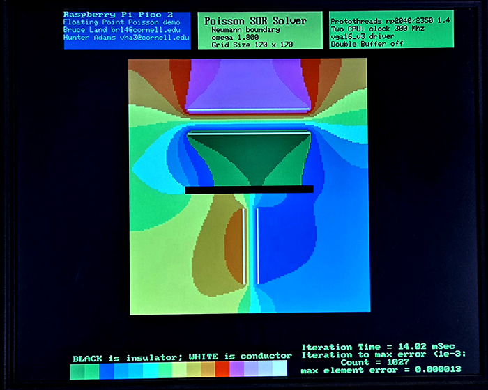
This example defines a 170x170 compute grid, with Neumann boundary condition, and three internal structures. This geometry is the digital version of an analog electric field mapper we used in college, called Teledeltos paper. The physical model for this simulation is a 2D, square array of equal-value resistors, with each computational node having a resistor linking it to four neighbors. If the edges of the finit array are unconnected, then the boundary condition is a Nemann condition with no current flow out, and therefore zero normal gradient. If the edges are connected to the same constant potential, then the boundary condition is an isopotential Dirichlet condition. Isopotential nodes inside the array are fixed voltage sources. Insulators inside the array simulate cut connections between nodes. The source term of the Poisson equation is modeled as nodes to which a fixed current is applied.

Near the top of the grid there is a pair of horizontal parallel isopotential lines (white) held at different potentials, to simulate a parallel-plate capacitor. The different color isopotentials squeezed between them expand out at he edges. In the middle there is a black rectangle which indicates a region of insulating material. At the edge of the rectangle, and the Neumann boundary, isopotentials must be perpendicular to the boundary. Near the bottom there are two vertical lines of isopotentials. The count indicator near the bottom right shows that it took 1027 iterations to reach a max error of 0.001 with omega=1.80. The color bar at the bottom shows the map of voltage to color, black is zero, yellow is 8, and white is 15.

Code, ZIP with all dependencies

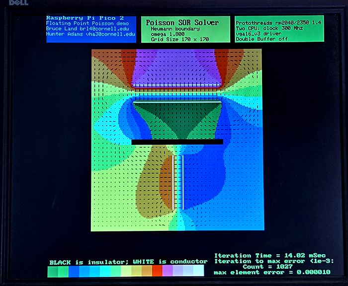
Using the field command superimposes an estimate of the gradient vector field on the image.
Note that the vector directions are correct, but the magnitudes have been partially normalized.

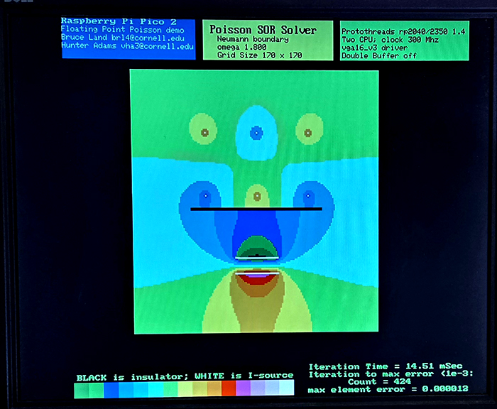
Example program with current sources and insulator,.
This example has six current sources with balanced positive and negative currents.
Below the sources is an insulator, and below that short, parallel line sources.

Code (use above ZIP and modify cmakelists to point to this code)

Example advecting a particle through the field.
The vector field, E, related to the potential is computed as the gradient of the potential.
The gradient is approximated as the centered difference of the potential in the x and y directions.

E_x = k*(u_i+1,j - u_i-1,j)
E_y = k*(u_i,j-1 - u_i,j-1)

Where k is a constant which merges test-particle charge and integration time step.
A k in the range of 0.05 to 0.20 seems to give good animaation rate.
The x and y components represent a force which are then separately Euler-integrated
twice to get the updated particle position.

There are three added serial commands:

• parton -- turns on the particle tracer
  -- default initial conditions x=85, y=85, vx=0, vy=0
• partoff -- stops the particle trace
• part x y vx vy -- sets initial conditions for the particle
  -- with 1<x,y<174 and -2.0<vx,vy<2.0

Code (use above ZIP and modify cmakelists to point to this code)

Copyright Cornell University April 23, 2026