Introduction top
"A MATLAB-based hearing test capable of mapping a user's hearing"
For our ECE 5030 final project, we present a MATLAB-based hearing test capable of mapping the frequency response of the user’s hearing. We achieve this by slowly increasing the amplitude of a given frequency and having the user press a button when they can hear the tone of the frequency under test. This procedure is iterated 23 times to fully map the user’s hearing over the entire human hearing range. Our system is modular in the sense that only a pair of headphones is needed to map your hearing. In addition to the standard hearing test where frequencies are played through both headphone speakers, we have also added the ability to test single ears. Finally, our system is capable of playing masking frequencies while simultaneously taking the hearing test to measure the effects of masking frequencies on the user’s overall hearing. Possible applications of our system include:
1. Medical: Used to detect various forms of hearing disabilities and build custom hearing aids and implants.
2. Communication: Used in Audio/speech compression and coding for storage and transmission. Eg. MP3 and AAC.
3. Consumer Products: Personilized Equilizers for music players, Sound Enhancement applications for mobile devices.
High Level Design top
Motivation
Throughout the lectures and labs in ECE 5030, we learned how to record physiological data from places such as muscle and the heart. We learned to record with not only traditional electrodes, but with optical IR sensors as well. While we found this work interesting, we wanted to do something new for our final project. During our initial brainstorms, we realized that we had not covered material related to the human ear, so we figured that doing a project related to hearing could be a great opportunity to learn more in the area of bioinstrumentation.
Background
The figure below shows the perception of human hearing between 20Hz and 20kHz.
Perception of Human Hearing between 20Hz and 20kHz (1)
Psychoacoustics is the scientific study of sound perception. Sound waves that propagate through the air as a vibration are picked up by the ear and converted to neuron action potentials. These neuron potentials are processed in the brain and perceived as sound. The human ear can perceive sounds in the frequency range of 20Hz to 20kHz. A minimum threshold level is required for a frequency to be perceived by humans. The minimum threshold is not constant across the frequency range and is known as the auditory threshold. The human hearing is most sensitive between 1000 Hz and 2000 Hz. Another phenomenon explained by psychoacoustics is Simultaneous Masking. Simultaneous masking occurs when a sound is made inaudible by a noise or unwanted sound of the same duration as the original sound.
The aim of our project was to build a system that could map the hearing threshold of a test subject, as well as show the effects of a masking frequency on the hearing threshold.
Background Math
The intensity of the auditory threshold is usually represented as a sound pressure level, measured logarithmically in SPL dB. The sound intensity I may be expressed in decibels above the standard threshold of hearing I0. the expression is:
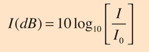
Mathematical Expression for Sound Intensity in Decibels (1)
For our project, we used a sine wave with I0 = 0.01 mV, corresponding to 0dB. The subsequent values are 1.2 times the previous voltage.
The frequency sensitivity of the ear is also non-linear and is typically represented with a logarithmic scale. The frequencies we selected are separated by a factor of 1.2 (approx.). We acquired the thresholds for the frequency set [90 133 200 300 445 666 1000 1200 1440 1730 2075 2490 2985 3583 4300 5160 6190 7430 8920 10700 12840 1540 18490].
Overview
Introducing our system with a high-level block diagram, we can see that there are three major components. These components are the PC running MATLAB, the headphones, and the user. The control flow starts with MATLAB, where frequency tones are generated at specific amplitudes and output through the headphone jack to the pair of headphones. The user wears the pair of headphones and is able to hear the frequency tones generated once they reach a particular intensity. When this intensity is reached, it is the user's job to hit the feedback button on the MATLAB GUI.
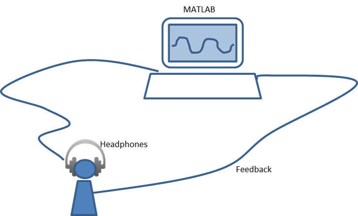
A High Level Block Diagram of our Audio Mapping System
Instructions for Use
1) Press the Windows key to bring up the Windows Start Menu.
2) In the search for programs and files box, enter "sound" then select "Sound" under the Control Panel option.
3) In the sound menu, scroll down to the headphones option, then right click and select properties.
4) Click the levels tab and slide the slidebar up to 80.
5) Open either our regular test or the test with masking with MATLAB, then click the run button.
6) When ready, click the start test button on the GUI, and hit the feedback button when a frequency is audible.
Hardware/Software Tradeoffs
Our project did have some initial design decisions to make between implementation in hardware or software. Although a trivial item, a large decision we had to make was whether to implement the feedback button in hardware or software. While we thought it would be beneficial to have the user click a physical button when they could hear a tone, we decided instead to implement this functionality through a software button. The reason for this decision being it seemed silly to introduce a NIDAQ and a push-button into our system when the rest of the project was completely implemented in software. This would mean that people who wish to use our system would need to have a custom board or button and a NIDAQ, as opposed to simply having MATLAB. We also initially had a board to do some simple filtering on the output of the audio jack, but we determined that the noise on the line was small enough to be ignored, given the ability to again keep our system a strictly software solution.
Software top
Overview/Program Design
Code Flow: The algorithm begins at low frequencies at an intensity level that is inaudible. The intensity increments at every iteration until the test subject can hear the tone. When the tone is audible by the test subject, he/she clicks the feedback button. Upon clicking the feedback button, the amplitude of the current tone is recorded and the next frequency is selected. The process is then repeated until the last frequency in the buffer has been played.
A listing of actions is:
1. Initialize amplitube and frequency buffers and set the minimum amplitude.
2. Select frequency and set amplitude = Minimum amplitude.
3. Increment amplitude = 1.2*amplitude
4. Create a sine wave of selected frequency with ramp up and ramp down.
5. Play the sine wave for 1 second.
6. If no feedback, go to step 3, else continue.
7. Record the amplitube for the selected frequecy.
8. If all frequencies are not done, go to step 2, else continue.
9. Plot the data and fit a 6th order polynomial curve.
Logical Structure: Flow Chart
we may also visualize the control flow of our code via the following flow chart:
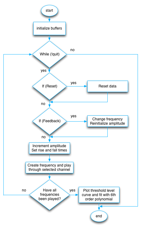
Software Flow Chart
Interface
A brief description of the testing graphical user interface (GUI).
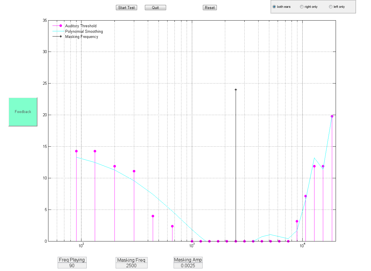
Screen Capture of our Graphical User Interface
Start/Pause Test Button: This button can be used to start or pause the test at the will of the test subject.
Quit Button: Quits the test. The program automatically saves the data of competed tests as a MAT file.
Rest Button: Resets all the data acquired and allows the subject to restart the test.
Mode Selection: The subject can select Both ears (mono), left ear, or right ear as the mode of the test. This allows the subjcet to test both ears or each ear seperately.
Feedback Button: This button is used by the subject to record when a frequency is audible. The system records the amplitude and moves on to the next frequency.
Frequency Box: Indicates the current frequency being tested.
Masking Frequency Box: Present only in the masking test. It allows the the subject to set the masking frequency in Hz.
Masking Amplitude Box: Present only in the masking test. It allows the the subject to set the masking amplitude in V.
Plots: The Stem plot indicates the amplitude level of the test frequencies. The cyan line is the polynomial fit line. After the completion of the test, the data points are connected and the polynomial fit curve is also plotted. The color of the plot and polynomial fit is set to blue for both ears, red for the right ear and green for the left ear.
Masking: To show the effects of masking, the sine wave is generated a combination of a masking frequency and the test frequency. The same procedure is repeated to obtain the threshold curve with masking. We have obtained data for masking at 500hz, 900Hz, 2500Hz and 6000Hz. The frequency and the amplitude of the masking frequency can be entered in the appropriate text boxes at the bottom of the interface
Optimization: The test takes more than 15 minutes to complete if the amplitudes start at 0.01 mV for all frequencies. Since the threshold mapping is non-linear, the time per test can be reduced to about 5 minutes per test by optimal selection of the starting amplitudes of different frequencies. The ides is to set the starting amplitude to less than the audible amplitude at that frequency. The amplitudes were selected by trial and error such that the time taken for each frequency to become audible is almost constant. The starting amplitudes are selected as:
| Frequency (Hz) | Starting Amplitude (V) | Starting Amplitude (dB) |
|---|---|---|
| 90 | 0.000266233 | 14.25262 |
| 133 | 0.000266233 | 14.25262 |
| 200 | 0.00015407 | 11.87718 |
| 300 | 0.000128392 | 11.08538 |
| 445 | 0.0000248832 | 3.959062 |
| 666 | 0.00001728 | 2.375437 |
| 1000 | 0.00001 | 0 |
| 1200 | 0.00001 | 0 |
| 1440 | 0.00001 | 0 |
| 1730 | 0.00001 | 0 |
| 2075 | 0.00001 | 0 |
| 2490 | 0.00001 | 0 |
| 2985 | 0.00001 | 0 |
| 3585 | 0.00001 | 0 |
| 4300 | 0.00001 | 0 |
| 5160 | 0.00001 | 0 |
| 6190 | 0.00001 | 0 |
| 7430 | 0.00001 | 0 |
| 8920 | 0.000020736 | 3.15725 |
| 10700 | 0.0000515978 | 7.126312 |
| 12840 | 0.00015407 | 11.87718 |
| 15410 | 0.00015407 | 11.87718 |
| 18490 | 0.000953962 | 19.79531 |
Results top
Speed of Execution
The test takes approximately 5 minutes to perform a complete auditory mapping on the user. This average time holds true regardless of whether the user is taking a test on both ears, the left ear, or the right ear. This is also the same when taking a test with a masking frequency. This time can be either longer or shorter depending on the user’s hearing, as more time is needed if given frequencies need to be played for a longer amount of time. During our testing, we found the entire procedure took about 15 minutes to run the test on both ears, the right ear, and the left ear. Originally, the test took about 15 minutes to complete a single run, but to expedite this we start the baseline amplitude above 0 dB. Both lab partners measured the amplitude of each frequency that could be heard, averaged that value, and then subtracted 8 steps. This significantly increases the speed of the test. In more professional situations, a larger sample size should be used to set these thresholds.
Another important speed to note is the speed of our GUI. Overall, the GUI is very fast, but there exists delay between pushing buttons and having actions occur. This is due to a limitation with our MATLAB toolbox used to output our sinusoidal tones to the headphones. When a tone is playing, we are unable to do anything else. During our testing, we play tones for a second on loop, so depending on when in that cycle a button is pushed, there can be up to a maximum delay of one second before “something” happens. If a future user should change this parameter, then this delay can be reduced or lengthened.
Accuracy
In order to characterize the accuracy of our test, we decided to perform a repeatability test. One of our test subjects ran the same test three consecutive times. The results of these tests are shown below.
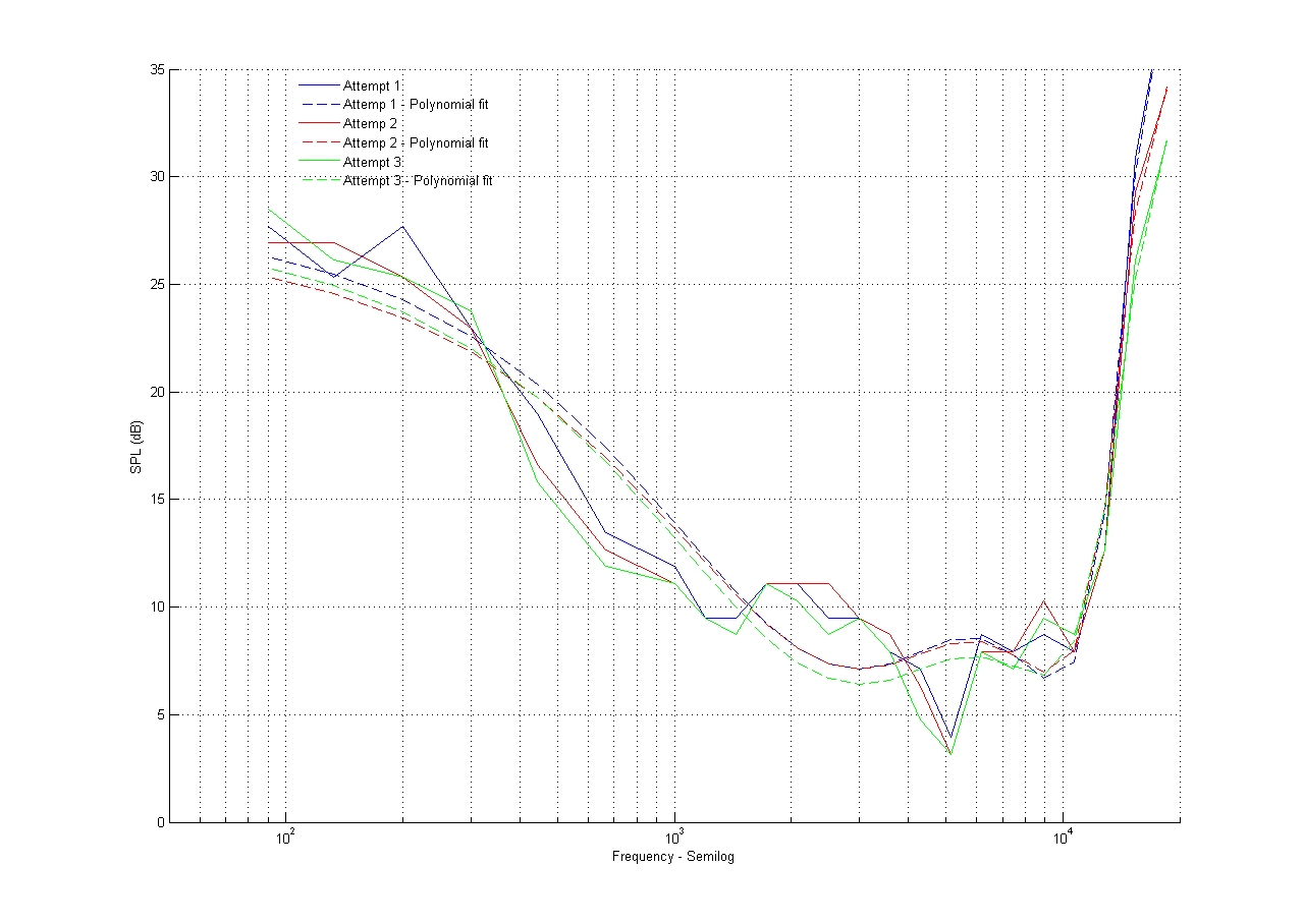
Repeatability Test Showing Differences between Taking Test 3 Consecutive Times (Subject-2)
From looking at the above figure, we can see that the test is very repeatable. Many of the data points are only one LSB away from each other, which is within the limits of human error. Some data points are multiple LSB's away, but this could be explained by environmental distractions that occured during the test.
How Did you Enforce Safety in the Design?
Safety was a key concept we kept in mind during the design and development of our system. We wanted to be able to create a safe method of testing human hearing and in order to do this, we limited the maximum amplitude output from the headphone jack of the PC. The maximum volume our system can output is 50 dB, which is a very safe volume to listen to. According to our source (4), volumes as loud as 85 dB are considered safe to listen to as long as the exposure is not longer than 8 hours per day, or 40 hours per week.
Interference with Other People's Designs
Another important thing to consider when designing a product is interference with other products or designs. Since our system is completely contained within a pc, and the generated tones output from the computer will stay within a closed loop between the headphones and user, we have determined our device to be safe around other products.
While our device is compatible with other forms of electronics, one thing worth noting is that our test is susceptible to the environment around the user. For example, when making our test on lab sessions that were full, we found the talking and noises generated from other groups and projects distracting and interfered with our test results. In other words, our test’s generated sounds are “masked” in a sense. Even when sitting in the lab when it was empty, we found that the ambient sounds of the environment, such as overhead fans or other pc’s had a non-negligible sound. The best solution to this problem is to take the test in a quiet environment with as minimal distractions as possible, or to take the test with high-quality noise-cancelling headphones.
Usability by you and Other People
A final consideration when designing our project was usability by others. The nice thing about our hearing test is that tones are “universal.” Regardless of what your native language is, you should be able to press a button when you can hear the tone. While our GUI is in English, it could be easily translated, and we have made the feedback button large and green. Users who have disabilities other than complete deafness should be able to take our test and map their hearing.
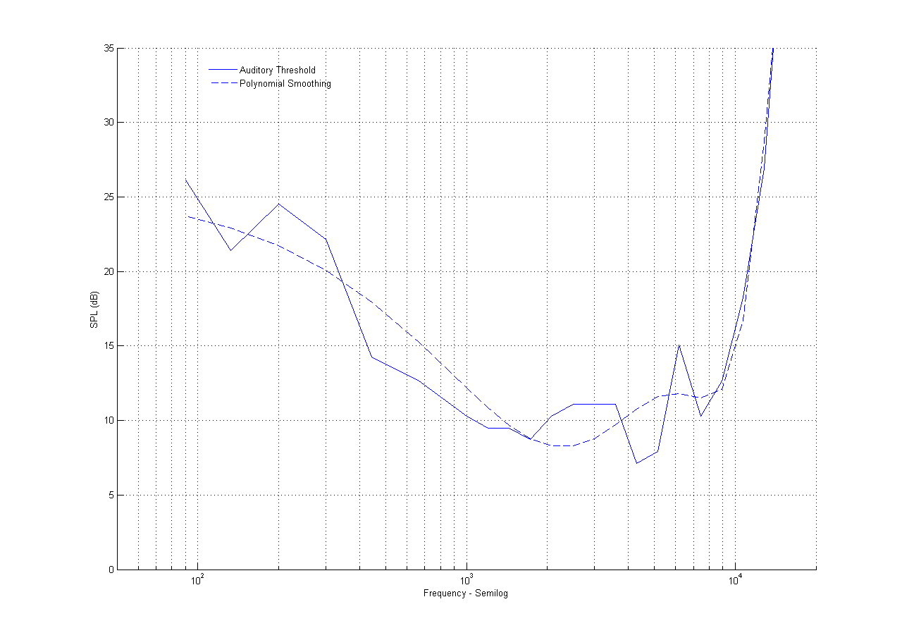
When testing our system with our subjects, we observed that the data taken from the first test was typically a bit “off.” We believe that this phenomenon is due to a learning curve associated with taking the test for the first time. To overcome this problem, we typically instructed our subjects to run through the first few frequencies as a learning trial, and then reset the test for the subject before logging the results. By viewing the figure below, you can see the results of one subject taking the test for the first and second time. It is easy to spot the discrepancies between the tests and we can also see that the results are much better for the second attempt.
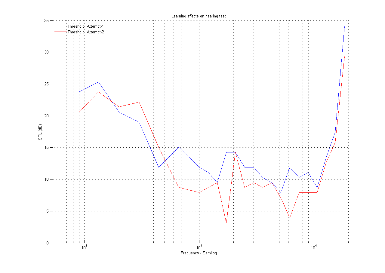
Subject-4 (20-30 years old) First and Second Trial Results showing Effects of Learning on Audio Mapping Test
Results
In this section, we will display the data we have collected with both our normal auditory threshold test and masking test.
Audio Threshold Results
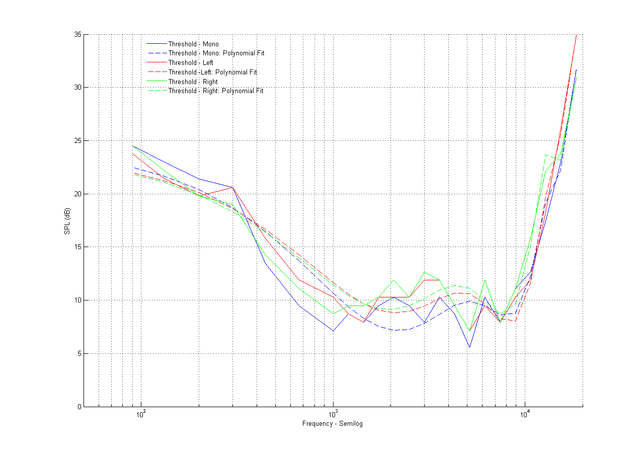
Audio Threshold for Subject-1 (20-30 years old)
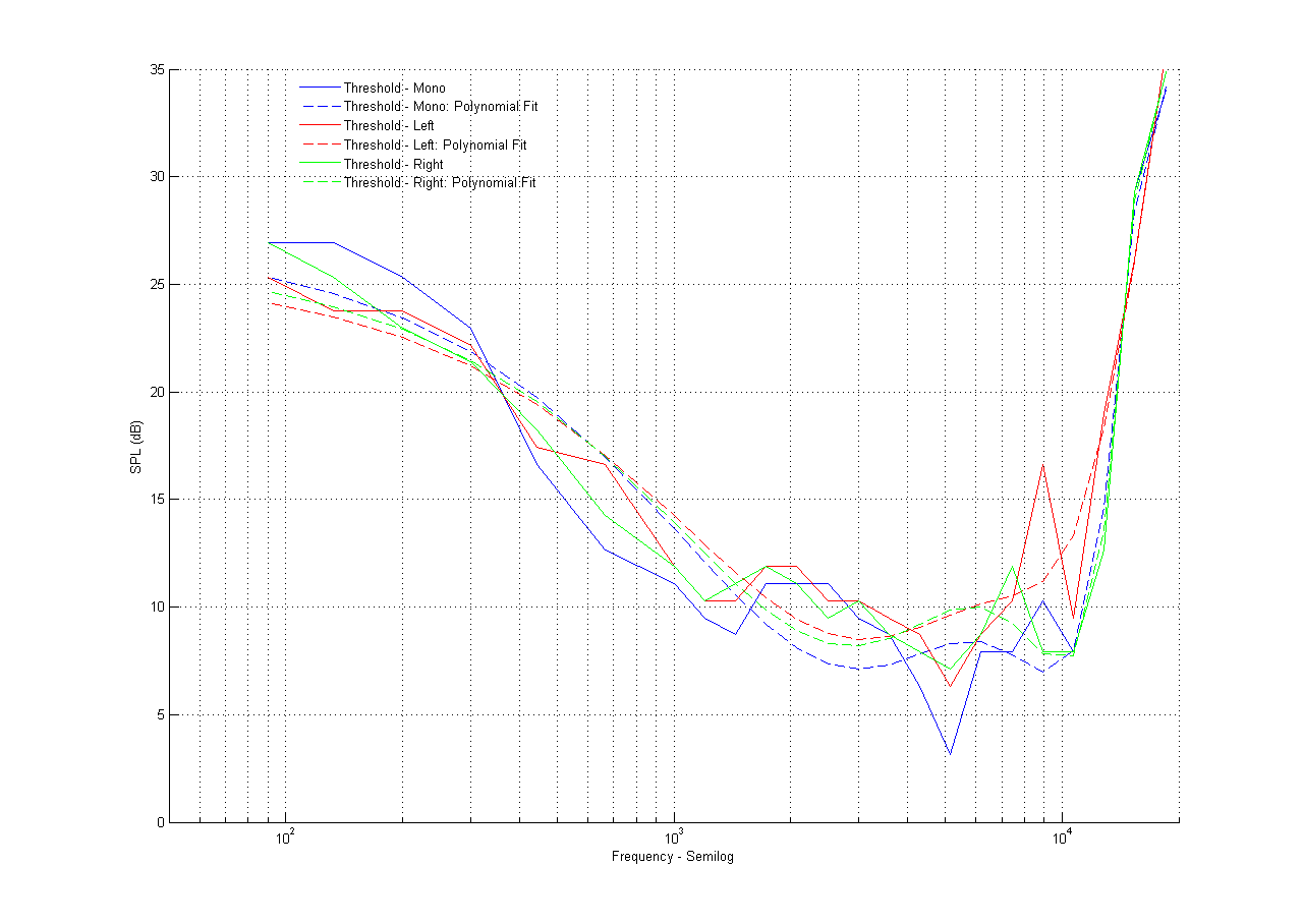
Audio Threshold for Subject-2 (20-30 years old)
The above two images show the relationship of the audio threshold between mono and left/right ear only. As expected, the results are very similar between tests. Comparing these results to literature (3), we can see that there is a strong similarity in the data to the typical human hearing response.
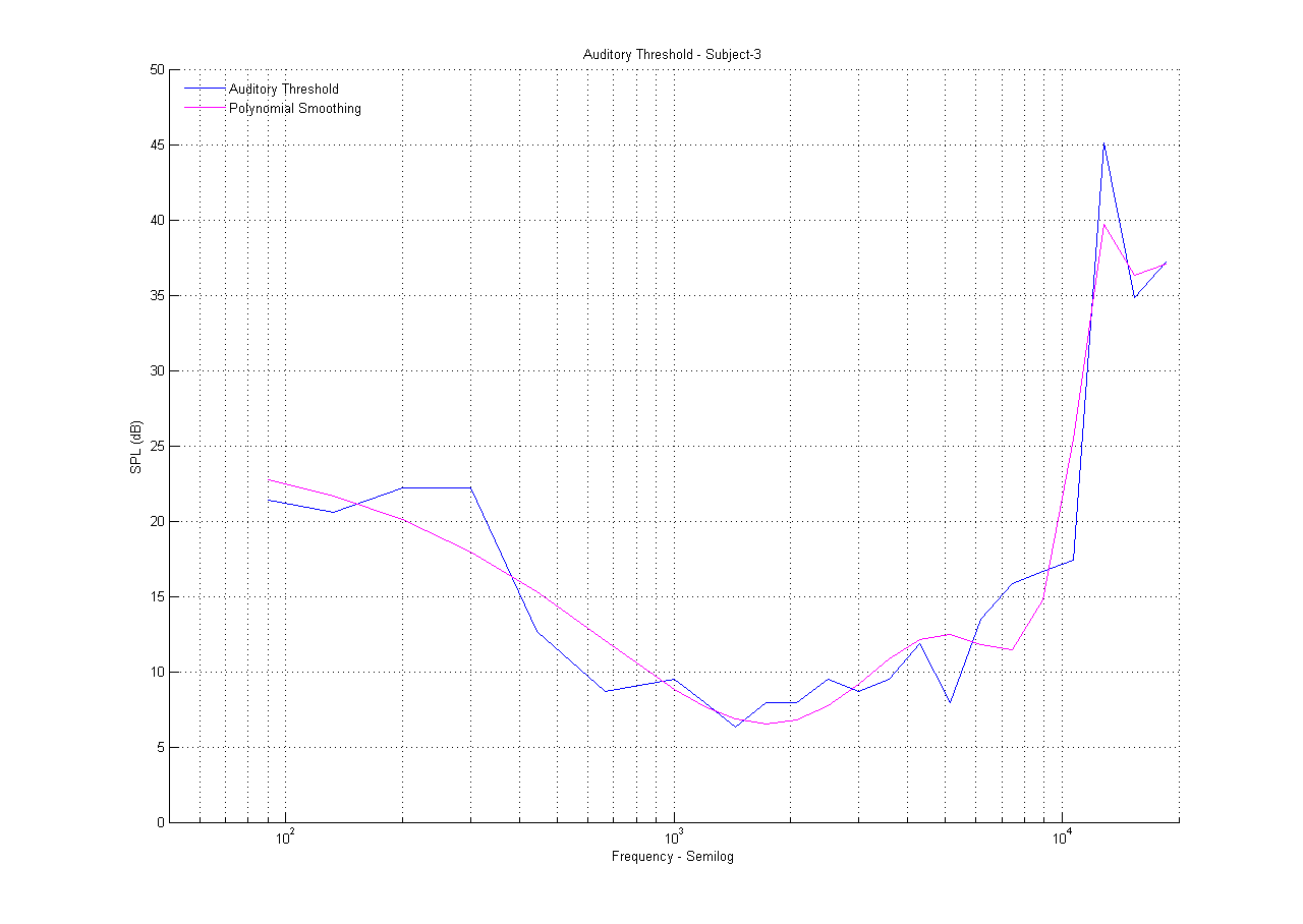
Audio Threshold for Subject-3 (60-70 years old)
In the above image, we can notice that the upper limit of audible frequencies tend to decrease with age.
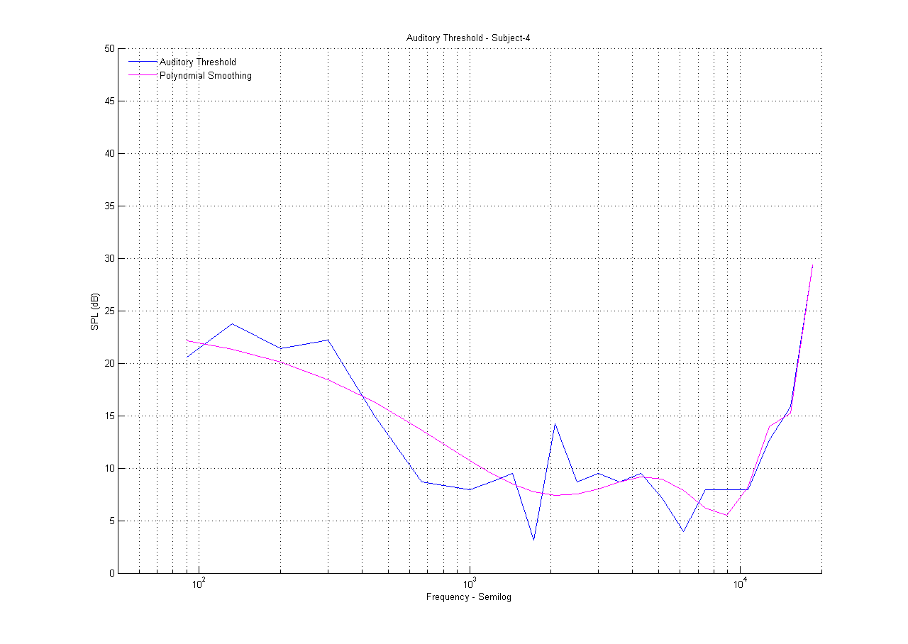
Audio Threshold for Subject-4 (20-30 years old)
Audio Threshold for Subject-5 (40-50 years old)
This subject is often exposed to loud sounds. It is interesting to see that the audio threshold is shifted upwards by about 5 dB compared to the other test subjects.
Masking Threshold Results
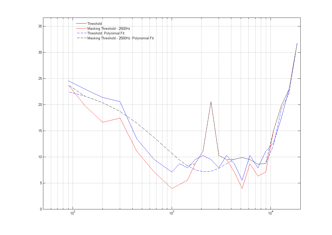
Audio Threshold for Subject-1 (20-30 years old) under Effects of a 2500 Hz Masking Frequency
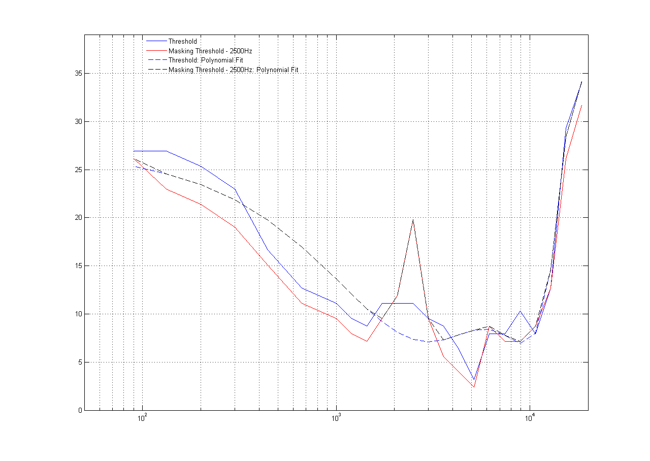
Audio Threshold for Subject-2 (20-30 years old) under Effects of a 2500 Hz Masking Frequency
Audio Threshold for Subject-3 (60-70 years old) under Effects of a 2500 Hz Masking Frequency
Audio Threshold for Subject-4 (20-30 years old) under Effects of a 2500 Hz Masking Frequency
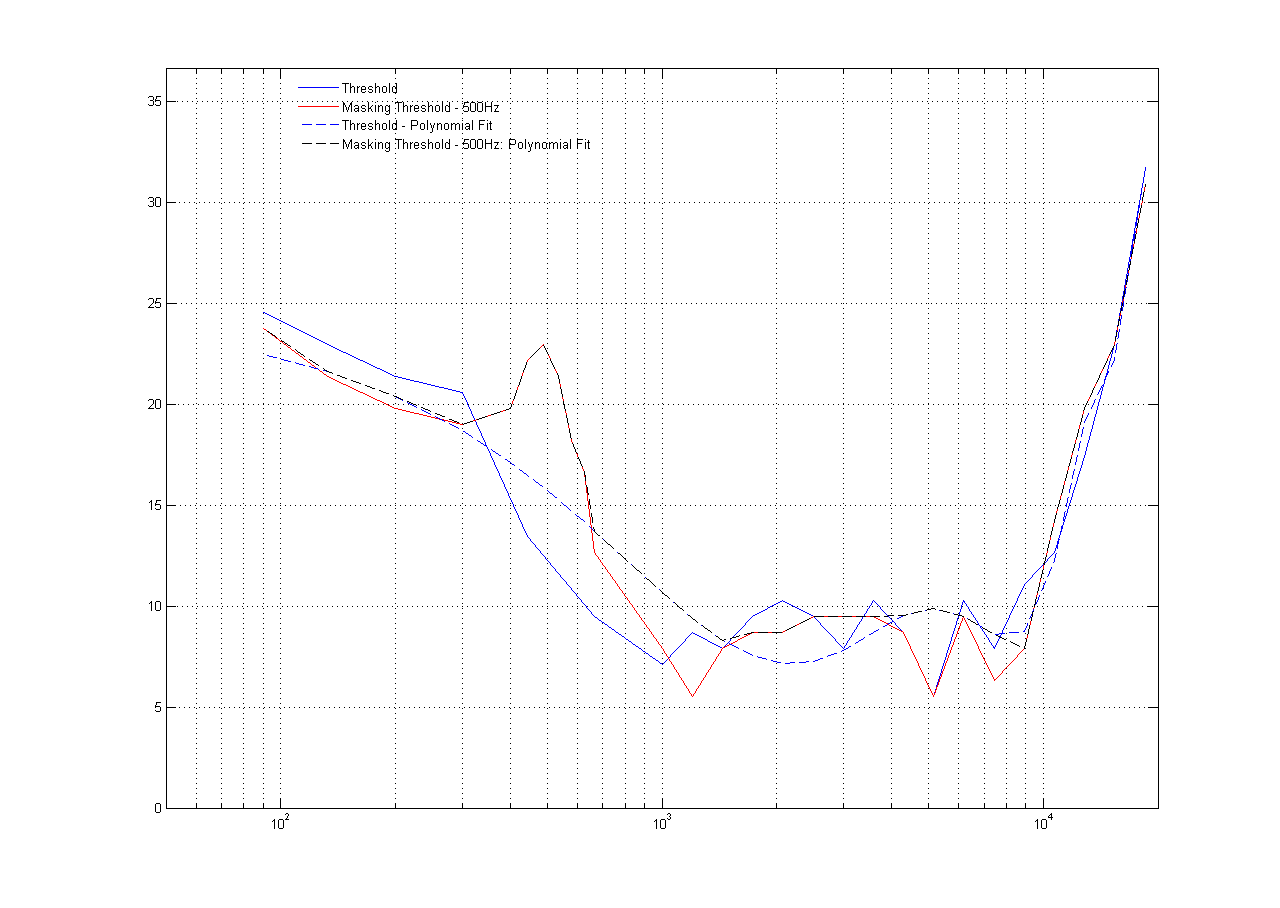
Audio Threshold for Subject-1 (20-30 years old) under Effects of a 500 Hz Masking Frequency
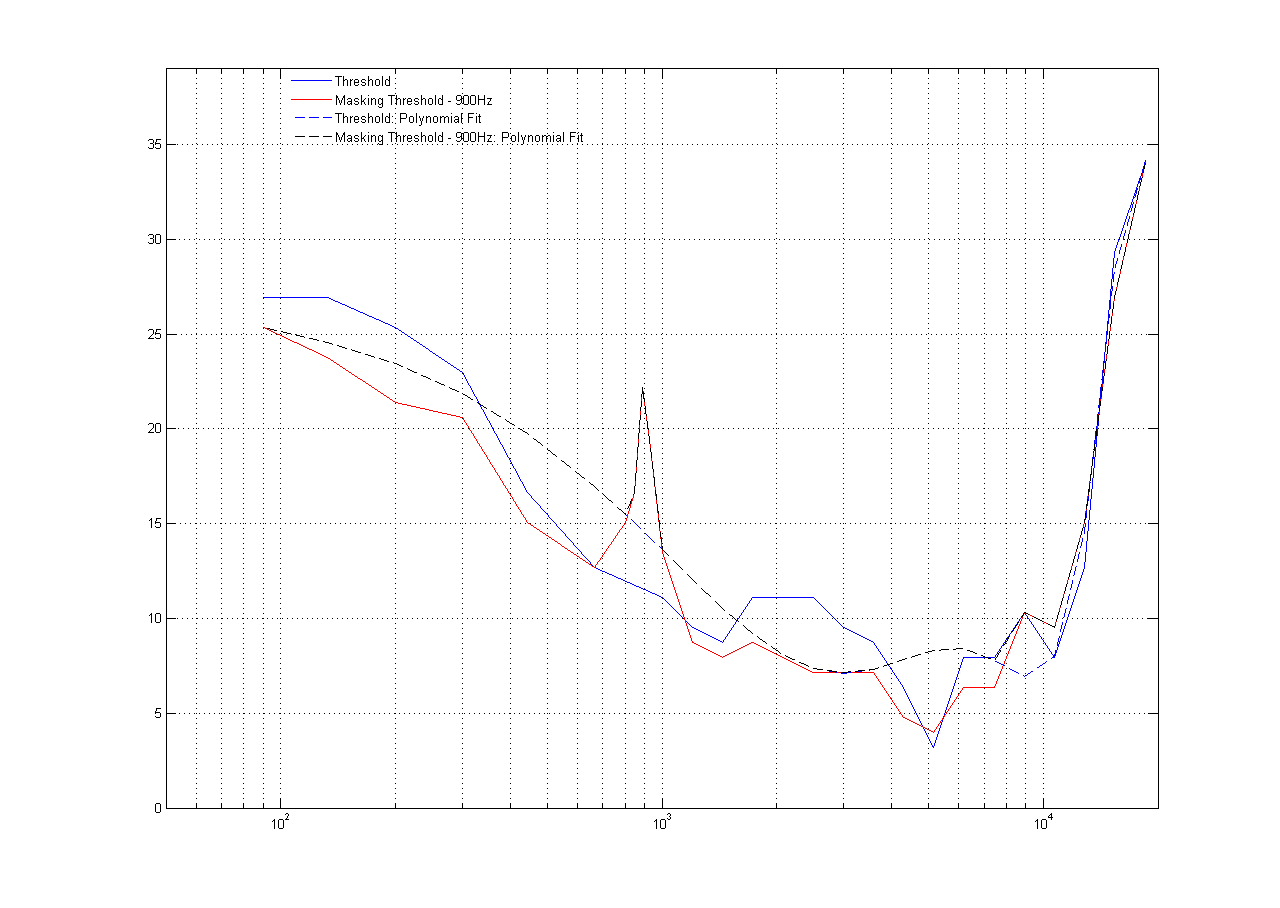
Audio Threshold for Subject-2 (20-30 years old) under Effects of a 900 Hz Masking Frequency
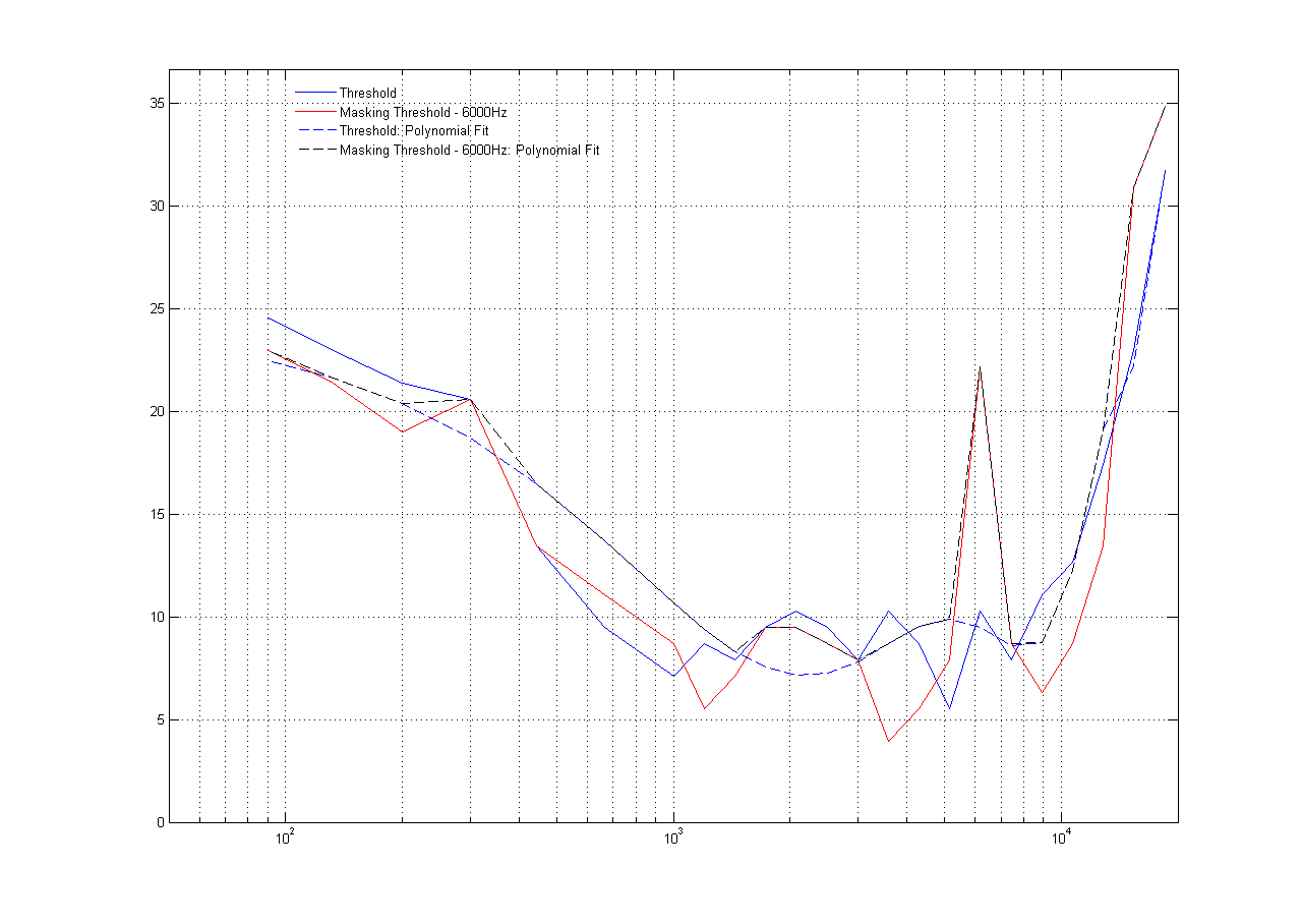
Audio Threshold for Subject-1 (20-30 years old) under Effects of a 6000 Hz Masking Frequency
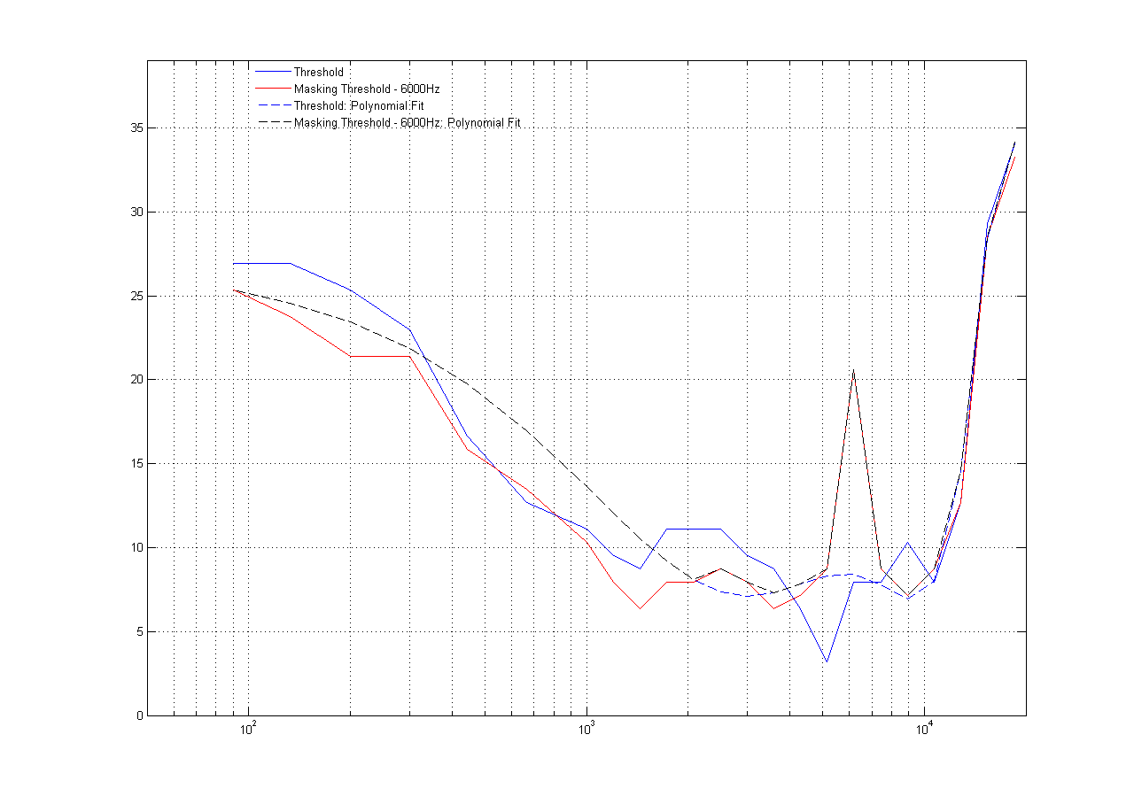
Audio Threshold for Subject-2 (20-30 years old) under Effects of a 6000 Hz Masking Frequency
The masking test results yield two important takeaways:
1. The audio threshold is higher around the masking frequency compared to the normal audio thresholding results
2. The bandwidth of the masking is not constant across all masking frequencies. The masking bandwidth is minimum for a masking frequency between 1000Hz- 2000Hz. It tends to increase for lower and higher masking frequencies.
Conclusions top
Summary
Overall, we consider our project to be a success. Our system achieves everything that we had originally wanted to do. It is able to map a user's hearing reliably, and is easy and convenient to use, since it is completely a software solution. In addition to the simple hearing test, we added a single-ear feature, where we are able to test the hearing in the user's right or left ear, instead of testing them both at the same time. Finally, we implemented a masking test, where the user can take the entire test with a baseline frequency playing in the background. We collected a lot of data from subjects of different ages, and drew a few interesting conclusions.
What Would you do Differently Next Time?
Given our experience designing this system, if starting from scratch, there would be a few changes we would make to our system. The first of these changes is implementing a feature where when the user hits the feedback button saying that they can hear the tone, the amplitude would then decrease on the same frequency and have the user hit the button again when they can’t hear the tone. We found that sometimes you think you can hear the tone, but then wait longer until you are sure that you can hear the tone. This puts some error on the results, and could be resolved with this proposed solution.
Similarly, we would like to add a feature to test a single frequency, as opposed to running the entire test. This way, if the subject hits the feedback button by accident, then they do not have to retake the entire test.
Another thing we would change is the MATLAB toolbox used to play the tones.We used the provided toolbox for our course, which is unfortunately limited to working on the 32-bit version of MATLAB R2010b. This forces users to have this particular version of MATLAB to use our test.
Appendices top
A. Parts List and Costs
The only parts needed for this project were a pair of noise-isolating headphones. One group member owned a pair of Ultrasone HFI-450 headphones, which were used throughout the entire project. Similar headphones could be replaced without penalty.
B. Source Code
The source code for both tests can be found here.
C. Division of Labor
| Karthikeya Pandit | Richard Speranza |
|---|---|
| Sweeping Frequencies | Sinusoidal Tone Generation |
| Thresholding | Ramping |
| Plotting Results | Left and Right Channel Test |
| Masking Test |
Please note that the majority of this project was completeted pair-programming style and that many of the tasks not listed here were completed by both partners. This for example includes data acquisition, data interpretation, background math, etc.
References
Datasheets
- The frequency response of the Ultrasone HFI-450 Headphones can be found here