Cornell University
BioNB 441
Using Graphics
Introduction.
Graphics covers a huge area of different techniques. I will attempt to provide examples of all the Matlab high-level graphics functions I have found, as well as some examples of lower level functions. Graphics might be used in neurobiology for:
The following examples will use Matlab base functions (no toolboxes). Each of the examples represents a typical graphics use, but there are many options which are not explained below. Use Matlab help to investigate each of the functions.
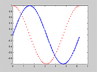
Simple x-y plot.
x=0:.1:2*pi;
y1=sin(x);
y2=cos(x);
plot(x,y1,'bx-',x,y2,'r.','linewidth',2);
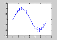
X-y plot with error bars
x=0:.4:2*pi;
y1=sin(x);
e=.3 .* y1 .* rand(size(x));
errorbar(x,y1,e)
set(findobj('type','line'),'linewidth',2)
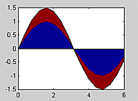
Area plot
x=0:.4:2*pi;
y1=sin(x);
y2=sin(x)/2;
area(x',[y1' y2'])
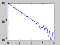
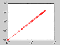
Log-log and semilog plots.
x=0:.1:4;
y1=exp(-x)+.01*randn(size(x));
y2=x.^2;
figure(1)
semilogy(x,y1,'bx-');
figure(2)
loglog(x,y2,'ro-')
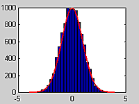
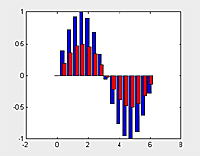
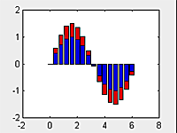
Histograms and bar charts
clf
data=randn(10000,1);
hist(data,30)
hold on
x_fit=-4:.1:4;
plot(x_fit, 1000*exp(-(x_fit.^2)/2),'r','linewidth',2)
x=0:.4:2*pi;
y1=sin(x);
y2=sin(x)/2;
figure(1)
bar(x',[y1' y2'],2)
figure(2)
bar(x',[y1' y2'],'stacked')
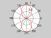
Simple polar plot
x=0:.1:2*pi;
y1=sin(x).^2;
y2=cos(x).^2;
polar(x,y1,'r-');
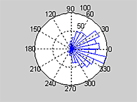
Angle histogram
theta=randn(1000,1);
rose(theta,30)
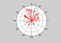
Vector plot at origin
x=0:.4:2*pi;
y1=sin(x);
y2=cos(x)+rand(size(x));
compass(y1,y2,'r')
set(findobj('type','line'),'linewidth',2)
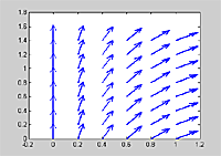
2D vector field as arrows
[x,y]=meshgrid(0:.2:1, 0:.2:1.5);
Vx=sin(x);
Vy=cos(x);
quiver(x,y,Vx,Vy)
set(findobj('type','line'),'linewidth',2)
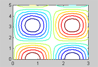
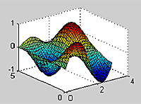
Contour plots, meshes and surfaces
[x,y]=meshgrid(0:.1:3, 0:.1:5);
z= sin(2*x) .* cos(y);
figure(1)
contour(x,y,z,10);
set(findobj('type','patch'),'linewidth',2)
figure(2)
meshc(x,y,z);
set(gca,'color',[.5 .5 .5])
figure(3)
meshz(x,y,z);
set(gca,'color',[.5 .5 .5])
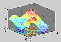
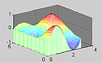
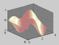
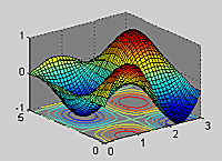
[x,y]=meshgrid(0:.1:3, 0:.1:5);
z= sin(2*x) .* cos(y);
figure(1)
surf(x,y,z);
figure(2)
h=surfl(x,y,z)
colormap(pink)
set(h,'edgecolor','none')
set(gca,'color',[.5 .5 .5])
figure(3)
surfc(x,y,z);
set(gca,'color',[.5 .5 .5])
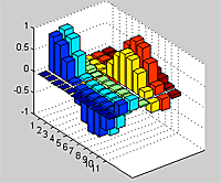
Bar chart
[x,y]=meshgrid(0:6, 0:10);
z= sin(x) .* cos(y/2);
figure(1)
bar3(z);
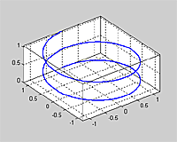
Simple x-y-z plots
t=0:.01:2*pi;
x=1.2*sin(2*t);
y=1.2*cos(2*t);
z=t/6;
plot3(x,y,z, 'linewidth',2)
grid on
box on
axis equal
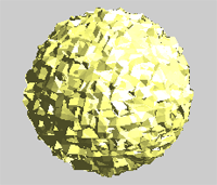
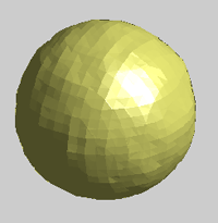
Isosurface determination of a 3D scalar field
clf
r=-1:.05:1;
[x,y,z]=meshgrid(r,r,r);
w=sqrt(x.^2 + y.^2 + z.^2)+0.02*randn(size(x));
isosurface(w,.5);
figure(1)
p=patch(isosurface(w,.5));
set(p,'facecolor',[1,1,.5],'edgecolor','none')
light
daspect([1,1,1])
axis off
view(30,30)
figure(2)
clf
w=smooth3(w);
p=patch(isosurface(w,.5));
set(p,'facecolor',[1,1,.5],'edgecolor','none')
light
daspect([1,1,1])
axis off
view(30,30)
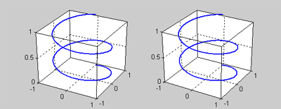
Streamlines and coneplot of a 3D vector field (and a stereo viewer)
clf
r=-1:.1:1;
[x,y,z]=meshgrid(r,r,r);
%generate a spiral velocity field
ux=5*y;
uy=-5*x;
uz=ones(size(x));

%=======================
subplot(1,2,2)

%make some streamlines
hs=streamline(stream3(x,y,z,ux,uy,uz,...
   r,zeros(size(r)),zeros(size(r))));
set(hs,'linewidth',2);

%attach some cones to the streamlines
spacing=30;
for i=1:length(hs)
   sx=get(hs(i),'xdata');sx=sx(1:spacing:end);
   sy=get(hs(i),'ydata');sy=sy(1:spacing:end);
   sz=get(hs(i),'zdata');sz=sz(1:spacing:end);
   hc=coneplot(x,y,z,ux,uy,uz,sx,sy,sz,2);
   set(hc,'facecolor','red','EdgeColor', 'none')
end

axis([-1 1 -1 1 -1 1])
box on
light('position',[10 10 10])
set(gca,'projection','perspective')
view(30,30)

%positions of the right eye
from=get(gca,'cameraposition');
to=get(gca,'cameratarget');
up=get(gca,'cameraupvector');

ax1=gca;

%===========================
subplot(1,2,1)

%copy the whole data structure to a new axis
copyobj(get(ax1,'children'),gca);

axis([-1 1 -1 1 -1 1])
box on
light('position',[10 10 10])
set(gca,'projection','perspective')

d=.5; %eye spacing
%get the position of the left eye
lefteye=from+d*cross((from-to),up)...
   /sqrt(sum((from-to).^2)) ;

set(gca,'cameraposition',lefteye);
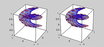
A stereo camera.
Draw all the objects you want in a view for the right eye, then copy the objects
into another axis and compute the view for the left eye. Only the computer graphic
camera position changes.
%define a 3D line
t=0:.01:2*pi;
x=0.9*sin(2*t);
y=0.9*cos(2*t);
z=t/6;

%===========================
subplot(1,2,2) %The right eye

plot3(x,y,z, 'linewidth',2)

% make the plotted region look nice
grid on
box on
axis([-1 1 -1 1 0 1])
set(gca,'projection','perspective')
view(30,30)

%positions of the right eye
from=get(gca,'cameraposition');
to=get(gca,'cameratarget');
up=get(gca,'cameraupvector');

ax1=gca;

%===========================
subplot(1,2,1) %The left eye

%copy the whole data structure to a new axis
copyobj(get(ax1,'children'),gca);

grid on
box on
axis([-1 1 -1 1 0 1])
set(gca,'projection','perspective')

d=.5; %eye spacing
%get the position of the left eye
lefteye=from+d*cross((from-to),up)...
   /sqrt(sum((from-to).^2)) ;

set(gca,'cameraposition',lefteye);
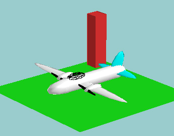
A hierarchical modeler.
Most of the information for this modeler is on a another
web page. The modeler allows you to construct elaborate 3D models and animate
them. One example image is shown below.
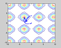
Computing and displaying trajectories.
The program below is a simple simulation of a 'butterfly' randomly searching
for regions of rich food sources. The trajectory is plotted as a series of dots
representing the butterfly. The butterfly has state variables of position and
velocity and is subject to small random accelerations. The butterfly is confined
to a 'cage' by reflective boundary conditions. The food distribution for this
simulation was periodic and is displayed as coutour lines of food density.
clf;

%initial butterfly position
x=0; y=0;

%initial butterfly velocity
vx=0; vy=0;
maxspeed=3;

%time step
dt=.1;

plot(x,y,'.')
s=10
axis([-s s -s s]);
hold on
set(gcf,'doublebuffer','on')

%build a food distribution and contour it
[foodx,foody]=meshgrid(-s:s,-s:s);
foodarray=((sin(foodx/2).^2+sin(foody/2).^2)/2).^4;
contour(foodx, foody, foodarray);
drawnow

for t=1:dt:1000

   %assume random accelerations
   vx = randn+vx;
   vy = randn+vy;

   %calculate current food and slow down if
   %food is plentiful
   food=((sin(x/2).^2+sin(y/2).^2)/2).^4;
   vx=vx*(1-food/2);
   vy=vy*(1-food/2);

   %impose a maximum flying speed
   speed=sqrt(vx^2+vy^2);
   if speed>maxspeed
      vx=vx*maxspeed/speed;
      vy=vy*maxspeed/speed;
   end

   %update positions and check for out-of-cage
   %reverse the velocity at the edges
   x = x + vx*dt;
   y = y + vy*dt;
   if x>s | x<-s
      vx=-vx;
   end
   if y>s | y<-s
      vy=-vy;
   end

   plot(x,y,'.');
   %text(0,-11,['t=',num2str(t)])
   axis([-s s -s s])
   drawnow
end