
I bet you guys could do a 64 point FFT with just combinatiorial logic!
Bruce Land
The Real Time Spectrogram project can compute and display the frequency spectrum of an audio signal on a standard VGA monitor.
The system uses an Altera DE2 prototyping board that contains an Altera Cyclone II FPGA. Audio is sampled using an onboard analog to digital converter at 8 kHz. The frequency spectrum is distributed linearly at a resolution of 32 frequency bins from 0 Hz to 4 kHz. The spectrum is computed with 32 bandpass filters and output to a VGA display in full color at 640 x 480 resolution. The interface consists of a scrolling spectrogram and a live magnitude bar graph.
This project was a five week design lab for ECE 576 at Cornell University.
Tim Schofield (tjs49)
Adrian Wong (aw259)
High Level Design
Fourier Transform | Discrete Fourier Transform | Fast Fourier Transform | VGA Display | HSL Color
The frequency content displayed on the spectrogram can be computed using two different methods. The first uses the Fourier transform and the second uses a set of bandpass filters. Both techniques were attempted in this project.
Fourier Transform
The Fourier transform maps a signal from the time domain into the frequency domain. The resulting frequency spectrum shows the frequency content of the original signal. The Fourier transform is based on decomposing a signal into an infinite set of orthogonal basis functions formed from the Fourier series. The specific mathematical details of the Fourier transform can be found in any number of reference texts online (e.g. Mathworld).
Discrete Fourier Transform
The Fast Fourier Transform makes use of a discrete-time, finite-domain Fourier transform known as the Discrete Fourier Transform (DFT).
The Discrete Fourier Transform is used for input signals that are both discrete in time and have a finite duration (finite domain). The audio codec on the DE2 generates a sampled waveform that is both discrete in time (samples are not continuous) and finite duration (waveform duration is finite).
The DFT transforms an input sequence of N complex numbers (x0, x1, ..., xn-1) into an output sequence of N complex numbers (X0, X1, ..., Xn-1). The DFT is given by Equation 1.
The exponential factor is often referred to as a twiddle factor and expressed with the following notation.
![]()
The DFT can be thought of as match filter that is convolving the input signal xn with an orthogonal set of sinusoidal basis functions given by the twiddle factors W(nk, N).
It should be noted that since the input sequence is real valued, the complex component of the input is always zero. As a result, the complex output frequencies of the DFT are symmetric about the Nyquist frequency (half the sampling frequency). For more details, please consider visiting reference texts regarding the Nyquist-Shannon sampling theorem and aliasing.
In the case of the spectrogram, the input sequence can be thought of as the set of real valued samples from the audio codec, and the output sequence is the set of frequency components of the signal. More concretely, let N be 64 and the sampling frequency be 48 kHz. This means that the input is 64 samples of the audio waveform, and the output is 64 equally spaced frequency bins of 750 Hz from 0 to 48 kHz. The frequencies from 24 kHz to 48 kHz are duplicates of the frequencies from 0 Hz to 24 kHz.
Fast Fourier Transform
The DFT is very computational intensive. As seen from equation one, each frequency component X(k) requires N complex multiplications and N complex additions. There are N frequency components, so an N-point DFT requires 2N2 complex operations (N2 multiplies, N2 sums). In big O notation, the DFT has a computational complexity of O(N2).
The Fast Fourier Transform uses several optimizations to reduce the number of operations to O(N log N).
Decimation (Divide and Conquer)
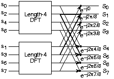
Decomposing a length 8 DFT into two length 4 DFTs.
(Source: Connexions)
One of the most important optimizations is decimation. For illustrative purposes, the radix-2 decimation-in-time algorithm shows how the DFT can be simplified to form an FFT.
The radix-2 DIT FFT algorithm starts by splitting the N-point DFT into two DFTs of length N/2. All the odd numbered indicies are grouped with one DFT and all the even numbered indices to another DFT.
This is called a radix-2 DFT because there are two groups, and it is called a decimation-in-time because the index of the time domain samples are the ones that are rearranged. There are also higher radix algorithms (such as radix-4) and also decimation-in-frequency algorithms (where the frequency bins need to be reordered).
With just one stage of radix-2 simplication reduces the number of complex operations to N + N2/2 complex multiplications and N2/2 complex additions. Recursively applying the radix-2 DFTs yields the O(N log N) result.
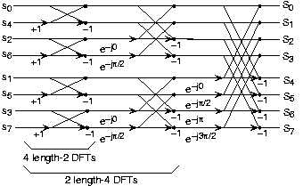
Further decomposition of the DFTs
(Source: Connexions)
Further savings can be obtained by moving to a radix that can more effectively computed on the FPGA. Radix-4 is especially useful, since the twiddle factors inside each DFT are just multiplications by ±1 or ±j.
Even more optimizations can be used with respect to the actual complex multipliers. See the radix-4 DFT implementation details for more information.
Bandpass Filters
The second method is to use a set of bandpass filters. These bandpass filters can be spaced linearly or logarithmically between the starting frequency and the Nyquist frequency. Each bandpass filter constitutes a single frequency bin in the spectrogram. The number of multipliers scale with the number of frequency of bins in the spectrogram as O(N).
VGA Display
Scrolling Video
A major component of our project is a smooth scrolling spectrogram that displays the magnitudes of 32 frequencies over an adjustable time window. At the beginning of our project, we realized we wanted our time window to be constantly updated rather than filled and then either frozen or cleared. However, we also had to consider that we most likely wouldn't be able to shift large chunks of video SRAM around at video rate during syncs, thus marking our first conceptual hurdle.
Instead, we began to think of the video SRAM as a circular vector of columns. We then realized that we could use some arbitrary pointer or offset to mark the beginning of the left most side of the screen, and use logic to cycle circularly through our vector. Thus, by moving offset at a fixed rate, we'd create a scrolling motion on screen. This concept is better illustrated in the diagram below.
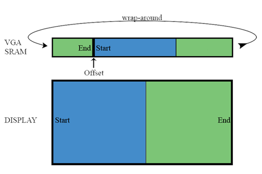
Treating video SRAM as a pseudo-circular vector of columns, with the leftmost portion of the screen marked by a moving offset.
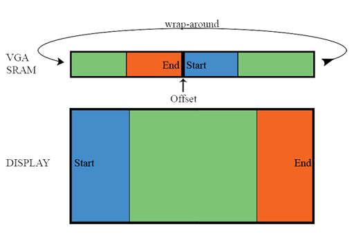
New data has been written into the SRAM vector at the old offset position, and the offset has been updated so that the newest input data appears on the right of the screen.
Treating the SRAM as a circular buffer of columns ensures that we would not have to shift SRAM data around, allowing for a quick, smooth scroll.
VGA Constraints
We decided early on that adjusting the VGA controller significantly would be beyond the scope of our project, which left us with the default screen resolution of 640 x 480 pixels, and a 25.2 MHz VGA control clock.
To see how many cycles we'd have per screen refresh, we used the sync information from http://www.epanorama.net/documents/pc/vga_timing.html. According to our source, each horizontal sync lasted 96 cycles, and each vertical sync lasted for 2 lines or 1600 cycles, for a total of 96*480+1600 = 47,680 cycles during which we could access SRAM.
The rate at which we updated columns in the spectrogram and moved the offset determines the apparent rate of scrolling. The desired rate of scrolling is also determined by the length of our window in both time and pixels. The read rate in clock cycles were determined by the formula:

HSL Color
Background
HSL color space is an alternative to RGB color encoding. H stands for hue, the aspect of a color that would be described by words like red, yellow, or blue. It is encoded as an angle from 0 to 360 degrees as shown in the following diagram.
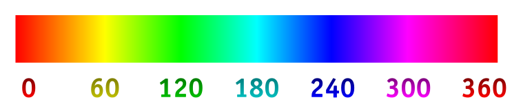
Image source: Wikipedia - HSL
S stands for the saturation of a color, a measure of the intensity of the color, or how much a perceived color differs from the color gray. L stands for lightness, is a measure of how bright a color is. Low lightness values lead to near-black colors, and high lightness values lead to near-white colors. The organization of the HSL color space is better shown by the following double-cone diagram.

Image source: Wikipedia - HSL
HSL color values can be converted to RGB values using the following set of equations:
Our HSL Color space
The major advantage to using the HSL color space in our project was that we were able to encode a broad and smooth range of bright colors without having to resort to a lookup table. This was achieved by using the 8 bit magnitude of each frequency as a hue value, and fixing the saturation value to 1 and lightness to 0.5 for the display of the spectrogram.
For our hue and saturation values, we calculated the q value to be 1, and p to be 0. We then multiplied all the formulas by 360 so we could avoid using fractions (and thus avoid the need to do any complex arithmetic in hardware). Finally, we scaled the Color result by the fraction 255 over 360 allowing us to convert to 8 bit values for each color for the VGA. The resulting equations needed only 1 multiply by a fixed factor for each color, followed by a right shift for a divide:
Implementation Details
Frequency Analysis: Radix-4 DFT | Hardware Tradeoffs | MATLAB | Verilog | IIR Bandpass Filters
Spectrogram Display: Spectrogram | HSL
Radix-4 DFT
Each radix-4 DFT module was modularized to take in four input samples, three twiddle factors, and four output samples. The complex additions and multiplications were further optimized in each FFT.
Each radix-4 butterfly requires three complex additions per sample for a total of 12 complex additions per butterfly. This can be optimized to use only 8 complex additions. Since each complex addition corresponds to two real additions, this means there are 16 real additions instead of 24 additions per butterfly.
Each radix-4 DFT has three twiddle factor complex multiplications. For each complex multiplier, this corresponds to two real adders and four real multipliers. This can be optimized to use five real adders and three real multiplications. As the multipliers require much more hardware than adders, this can result in a significant space savings.
The total radix 4 DFT hardware required was reduced from 30 adders and 12 multipliers for each DFT to just 27 adders and 9 multipliers.
Hardware Tradeoffs
Single cycle FFT
The original plan was to implement a single cycle FFT that could compute a 64 point transform in just one clock cycle of the 50 MHz system clock. This is even faster than the rate that the audio codec could put out samples (48 kHz). Theoretically, new samples would be shifted into the shift register and the 64 point transform can be computed as soon as the results cascaded through three stages of 16 DFTs.
However, the hardware requirements were too much. With 48 radix-4 DFTs operating in parallel, 288 multipliers would be required (the last stage of the FFT does not require twiddle factor multiplications). The Cyclone II FPGA used on the DE2 board (EP2C35) has only 35 embedded 18 bit multipliers and enough hardware to implement 105 soft multipliers for a total of 140 multipliers. The single cycle implementation would require slightly over 205% of the available logic area, or in other words, two EP2C35 FPGAs. This was verified when the compilation process failed when the fitter could not fit 64,000+ logic elements into the 33,216 logic elements available on the EP2C35. It should be noted for future reference that the 64 point FFT could be implemented by using a larger FPGA, such as the EP2C70 (400 multipliers, 68,416 logic elements). A smaller FFT could also be implemented on the EP2C35 by using a fewer number of points in the FFT and using less accurate 9-bit multipliers.
Multi cycle FFT
While there are still several optimizations that can be used to reduce the hardware requirements, the decision was made to transition to a multi cycle FFT.
In this configuration, the calculations are computed sequentially instead of in parallel. The amount of parallelization is variable, depending on how many FFTs are operating in parallel.
On one extreme is the fast single cycle FFT in which the 64 samples are cascaded through 48 radix-4 DFTs in a single batch. On the other extreme is the slow multi stage FFT in which 4 samples are processed at a time through a single radix-4 DFT in a sequence of 48 batches. In between both extremes are hybrid solutions where multiple DFTs compute the samples in stages. One example would be where 64 samples are processed through 16 radix-4 DFTs in 3 batches.
Each stage requires a finite number of cycles to retrieve the samples, calculate the DFT, and store the samples. Assuming a conservative estimate of nine clock cycles (three clock cycles to retrieve the samples, three clock cycles to calculate the DFT, and three clock cycles to store the samples), the slowest multi stage FFT would take 432 cycles (48 stages, 9 cycles/stage) to calculate a 64 point FFT. At a system clock of 50 MHz, this corresponds to an FFT speed of 115 kHz. This is still much faster than the 48 kHz rate at which the audio codec produces input samples for the FFT.
Thus, for an audio rate spectrogram, the FFT could operate without any DFTs in parallel. The total hardware required would be 27 adders and 9 multipliers. The tradeoff is the memory usage required to store, load, and keep track of which stage is being calculated.
Sequencing
If the FFT is computed sequentially, the correct samples and twiddle factors must be assigned to each DFT stage. This can be done by storing the incoming samples, twiddle factors, and the DFT results into memory blocks. An additional memory block can be created to store the appropriate indices for each memory block to compute the correct sequence of DFT calculations.
For a 64 point radix-4 FFT, there are 48 DFT calculations that need to be performed. For each DFT calculation, there are four samples that need to be fetched from RAM, three twiddle factors that need to be fetched from ROM, and four samples to store back into RAM. The index for the four incoming samples, three twiddle factors, and four outgoing samples can be stored in the sequencer ROM. The FFT state machine can increment through the sequencer, fetch the four samples and three twiddle factors, perform the DFT calculation, and store the four results. This process is repeated until the sequencer reaches the last entry in the sequence ROM. At this stage, all 48 DFT calculations have been computed and the resulting frequency data can be stored for future use.
There are also optimizations that can be made for the sequencer. The most immediate is to use an in place FFT algorithm. This is an algorithm where the indices of the incoming samples are the same as the indices used in the outgoing results. Thus, the incoming samples and the outgoing samples can be stored in the same RAM block, reducing the total amount of memory required. Additionally, the sequencer ROM now only needs to store one set of indices.
MATLAB Implementation
This implementation was tested in MATLAB first. The complex multipliers, radix-4 butterfly, and sequencer were all created in MATLAB scripts that approximated the future hardware implementation. The results of the FFT were compared with the MATLAB supplied FFT function and were found to have an exact one-to-one correspondence.
The MATLAB script for the sequencer was modified to automatically generate the Verilog code directly from the script itself. This allowed for very rapid automated Verilog code generation when parameters of the FFT were changed.
There are two MATLAB different implementations included in the appendix below. The first implementation was the one used to generate a 64 point single cycle FFT. The second implementation uses an in-place FFT algorithm. The two references (Tom Wada and Magnus Nilsson) were very helpful in development of the MATLAB scripts. Portions of the code structure are copied from the MATLAB scripts listed in the credits.
Verilog Implementation
The Verilog implementation was generated directly from the MATLAB scripts. For the creation of the single cycle FFT, the input and output wires must be named appropriately so that the correct values are passed onto each stage of the FFT. For the multi cycle FFT, Verilog code has to be written to correctly sequence the retrieval and storage of samples and twiddle factors.
The Verilog code for the FFT is contained within the fft64pt_seq module. The sample clock of the audio ADC, samples from the audio ADC, and handshake lines with the VGA are all inputs. The VGA display unit can request a specific frequency via a five bit address (32 distinct frequency bins) and receive the magnitude data in an unsigned 8 bit result.
The audio ADC shift register contains 64 registers that are 16 bit wide each. On each tick of the audio ADC clock, the shift register takes in the newest ADC sample (16 bits) and shifts the remaining samples over by one. The ADC shift register can be paused by the FFT state machine so that the samples do not change while the FFT state machine copies out the values.
The contents of the ADC shift register can be addressed externally with the audio sample address. The ADC sample at that index is read out and optionally passed through a windowing function. The windowing function multiplies the ADC sample by the appropriate scaling factor before sending the result to the FFT state machine.
There are three M4K blocks used by the FFT state machine. The first is the signal RAM that contains the 64 samples of data used in the FFT process. The second is the twiddle factor ROM that contains the twiddle factors used for each DFT stage. The third is the program sequence ROM that contains the indices into the first two M4K blocks for each DFT calculation.
The signal RAM is a two port RAM to maximize data bandwidth. There are two inputs of 36 bits each. Each input contains two signed 18 bit values representing the real and imaginary component of each complex number. The same format applies to the signal RAM outputs.
There is a series of multiplexers that control the data flow into and out of the signal RAM. The RAM can store or load two complex numbers at a time. The input of the signal RAM comes from either the ADC shift register or the DFT output. The output of the signal RAM goes to the DFT input or to the VGA display.
The FFT state machine choreographs the complex interaction between the program sequencer, signal RAM, twiddle ROM, ADC shift register, and VGA control block. Generally speaking, the FFT state machine can be split into four states: hold, load, store, and sample.
During the hold state, the FFT can be halted by the VGA controller so that the VGA controller has access to the signal RAM. If the FFT is not being halted, the state machine checks to see if new samples need to be acquired (sample state). If the samples have been written into the signal RAM, the FFT jumps to the load state. The DFT sequence counter is incremented, so the program sequencer can load up the indices required for the DFT calculation. The signal samples are retrieved from the signal RAM two samples at a time. The twiddle factors are retrieved from the twiddle ROM. The actual DFT calculation occurs in combinatorial logic, so the transformed values are ready in a single cycle. The signal samples are then stored back into the signal RAM. The DFT counter is incremented and the whole process is repeated until all 48 DFTs have been calculated. For the sample state, the FFT state machine overwrites the contents of the signal RAM with the 64 samples stored in the ADC shift register.
The actual DFT is modularized in the radix4dft. The complex multipliers are modularized in optcomplexmult. The optimizations used for each are recorded in the comments of the Verilog file.
Bandpass IIR Filters
The bandpass filters are fourth order IIR elliptic filters. The filter modules are from the ECE 576 course page and are fully modularized to use signed 18 bit fixed point notation. There is additional code in the MATLAB files that generate the filter tap weights. These MATLAB scripts were modified to generate 32 bandpass filters that can be spaced either linearly or logarithmically across the sampling frequency spectrum. Furthermore, the MATLAB scripts were modified to automatically perform the necessary scaling coefficients. Each filter uses one 18 bit multiplier. The complete set of bandpass filters uses 32 embedded 18 bit multipliers.
Spectrogram
The first step in implementing the spectrogram was controlling the rate at which we read the frequency inputs and copied them into display SRAM. We opted to use a 32 bit accumulator that operated at VGA CTRL CLK rate in order to determined when to sample and update. Whenever the accumulator was equal to or greater than the value (CLK * T / X), we would read the frequencies at the next opportunity and subtract (CLK * T / X) from the accumulator. In our final iteration, the time window was selectable using switches 2-0, which were hardwired to constants representing a window of 2 seconds through 9 seconds. The sampling constants were hardwired to avoid using up multiplier units.
Next, we required a state machine that would assert control over the registers containing the frequency magnitudes, blocking them from being overwritten, and read them into a buffer. During the vertical sync, this buffer is read and copied into SRAM, updating the pointer offset value after each column is copied in. We had more than enough cycles during the vertical sync to copy 6 samples of 32 frequencies each into SRAM.
This frequency copying state machine is outlined in the diagram below:
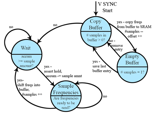
The VGA Frame state machine reset by a vertical sync.
After we had created our state machine, we needed logic added to the pixel blasting component of the VGA that would redirect the SRAM address being read based on the horizontal offset and frequency binning. We opted to use a spectrogram of size 600 x 256 pixels. We needed to display 32 distinct frequency bands, which meant each band would be 8 pixels tall. Rather than write each frequency's magnitude 8 times in SRAM, we simply ignored the lower 3 bits of each Y coordinate that fell within the spectrogram display.
We decided to display a bar graph of the magnitudes of the last frequencies stored to video memory for each video frame, similar to what can often be seen on an audio equalizer. We achieved this without having to perform any additional writes to video memory. Instead, we defined a region of 512 x 128 pixels (32 bars of maximum height 128 pixels, 16 pixels wide each) that would be dedicated to these bar graphs, and used the magnitudes stored in the last entry of the frequency buffer to determine the height of each bar.

Redirection of SRAM based on screen height of the pixel during pixel blast.
Each bar's height is set using the upper 7 bits of frequency magnitude stored in the buffer, and we once again use address redirection during a pixel blast if the pixel being addressed would be above the bar, and therefore black, we address SRAM normally, and if the pixel is part of the bar, we address the appropriate segment of the last column written into the spectrogram portion of video memory. Thus, we achieve additional display functionality at no cost in terms of data that needs to be written to SRAM.
Testing
First we tested our scrolling concept by drawing a white diagonal line on a black background in SRAM on a reset, and added logic to adjust a horizontal offset on each vertical sync, and to adjust the memory location addressed by the VGA controller by the offset amount. Our quick and dirty test proved the concept would work and generated a very smooth scroll with little needed in the way of logic.
Second, we tested our ability to put frequency information into display memory by creating a random bit generator and constantly copying 8 bit chunks of its output into a series of 32 registers. These registers would hold their value if a hold line was asserted, and could be addressed and read by our display state machines using a large 32 to 1 multiplexer. Our testing showed that we could read a stream of meaningless inputs fine, but also revealed a problem in our display. Initially, reads were written directly to SRAM, which resulted in the spectrogram getting updated mid-frame. This created screen artifacts in the form of horizontal lines rising upwards, and was visually distracting. To fix this problem, we created our buffer of frequency magnitudes and only copied into SRAM on the vertical sync. This resulted in smooth performance, but constrained our viewing window to a minimum of 2 seconds.
Next, we implemented the bar graph functionality and replaced our random input with fixed levels. This revealed some addressing errors in the display redirecting logic, such as frequency bins reading from the wrong input. These errors were corrected, and the display was once again working.
Our final version of the display component operated at a smooth 60 Hz frame rate and could display 32 frequency magnitudes in a spectrogram over a selectable time window from 2 to 9 seconds, with an accompanying bar graph of the most recent input.
HSL Implementation
The HSL equations were implemented as a stage between SRAM data and the VGA color inputs using combinational logic and registers. The conversion added 1 cycle of delay between the SRAM data and VGA color inputs, so we had to modify the VGA controller to address SRAM one cycle earlier to compensate.
Testing
We tested our HSL color space by simply writing a linear sweep of hue values from 0 to 255 in SRAM on a reset. The resulting image was a smooth transition from red to green to blue however, red corresponded to a 0 in SRAM, so we had to add a simple subtraction to reverse the direction of our color range, thus placing blue in the low end and red in the high end.
Finally, we had to add logic to properly draw black to the screen in the areas that were not displaying frequency information. The resulting display had pleasant and vibrant color, making it more appealing to look at.
Results
For the most part, the combination of the band pass IIR filters and the display works well. Here you can see a few movies of a few kinds of audio inputs into our system.
The first is an example of speech, in this case a part of Ted Steven's infamous The Internet is a Series of Tubes speech, which dealt with network neutrality. (Original MP4 File)
The second video displays an image hidden in the Aphex Twin song Windowlicker. An image of a face was drawn in the frequency domain and converted back to sound you can see the bottom half of a head scroll by on our display. A spectrogram with a larger frequency range and higher resolution would have been able to display more of the image. (Original MP4 File)
Finally, we have a video of the spectrogram with a midi of a version of Twinkle Twinkle Little Star being played. This midi makes use of high pitched bells to play the melody, and you can actually pick out the notes as they are played in the song. (Original MP4 File)
The apparent lines in the display in all of these movies are artifacts from the camera, and not present when viewed in person. Our filters all have some overlap in their bands, which causes leakage between frequency bins in the output. This is particularly a problem with our low frequency band pass filters, and is illustrated well by feeding a sine sweep through our system. Also, the DC band was constantly saturated we are unsure if this is because of a DC signal on the output, or if there is a problem with its implementation.
Because our filters were IIR, sound pops (impulses on input) would permanently increase their output levels by small amounts. Also, when filters became saturated by an input that was too loud, they would not return to zero but instead remain saturated. Both these small offsets and complete saturation could only be fixed by resetting the system, which is less than ideal.
Conclusion
Overall, the spectrogram display worked very well, but the background audio processing did not have a functional FFT. While the current implementation of bandpass filters provides sufficient data for a graphic display, a working FFT implementation would use less hardware and would scale better with higher frequency resolutions.
While our spectrogram and bar graphs are smooth on the display, a more complete implementation of HSL color, with adjustable saturation and lightness, would provide broader and more interesting visualization options. Developing a higher resolution display would have also given additional visualization freedom.
IP Considerations
The project uses the Altera codebase for the VGA controller and audio codec controller.
Appendix
Division of Labor
Tim Schofield worked on the VGA controller, scrolling VGA display, live bar graph display, and HSL color space representation. Adrian Wong worked on the audio codec ADC, FFT implementation, and bandpass filter integration.
Credits
The IIR filters were from Bruce Land's DE2 examples. Background for the FFT came from the FFT project page of Professor Tom Wada from University of the Ryukyus. Additional mathematics references come from Magnus Nilsson's paper on FFTs.
Source Code
MATLAB
- FFT Generation - In Place
- FFT Generation - Combinatorial
- Radix-4 DFT
- Optimized Complex Multipliers
- IIR Bandpass Filter Generation
- Bruce Land - IIR Bandpass Filter
- Bruce Land - Signed Fractional Bit Converter
- Tom Wada - 64-point In Place FFT
