Speaker Recognition

The goal for our project was to be able to distinguish, in real time, between various speakers based only on audio input. In the literature, this problem is known as speaker recognition, or, more precisely, speaker identification. A good deal of progress has been made in this field, but it is still an open research topic, and by no means a solved problem. Speaker recognition is applicable to many fields, including but not limited to artificial intelligence, cryptography, and national security.

Human speech, when analyzed in the frequency domain, reveals complicated, yet well understood features, which can be used to indentify the speaker. These features are derived from the mechanics of speech generation, which we shall introduce briefly here. The treatment here will be greatly simplified, and the interested reader is encouraged to consult the references for a more complete introduction.

Speech begins with the generation of an airstream, usually by the lungs and diaphram.^[1] - a process called initiation. This air then passes through the larynx (voicebox), where it is modulated by the glottis (vocal chords). This step is called phonation or voicing^[2][3], and is responsible for the generation of pitch and tone. Finally, the modulated air is filtered by the mouth, nose, and throat - a process called articulation - and the resultant pressure wave excites the air.^[4].

As a consequence of this physiology, we notice several characteristics of the frequency domain spectrum of speech. First of all, the oscillation of the glottis results in an underlying fundamental frequency and a series of harmonics at multiples of this fundamental^[5]. This is shown in the figure below, where we have plotted a brief audio waveform for the phoneme 'ah' and its magnitude spectrum. The fundamental frequency (113 Hz) and its harmonics appear as spikes in the spectrum.

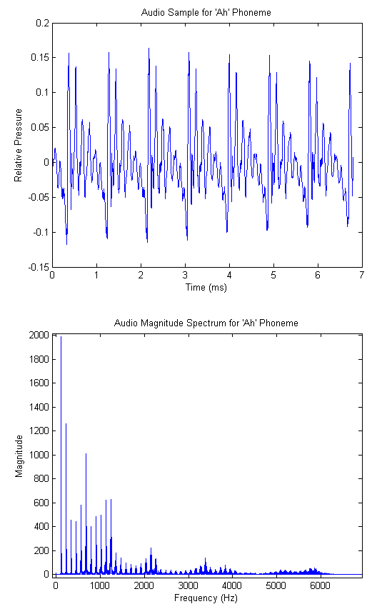
The location of the fundamental frequency is speaker dependent, and is a function of the dimensions and tension of the vocal chords. For adults it usually falls between 100 and 250 Hz, and females average significantly higher than males^[5].

Further analysis of the audio spectrum shows that nearly all energy resides in the band between DC and 4kHz, and beyond 10kHz there is virtually no energy whatsoever. Incidentally, this is one of the primary motivations for the common sampling rate of 8kHz. In our case, we wanted higher fidelity audio, so we chose the (more than suitable) sampling rate of 32kHz.

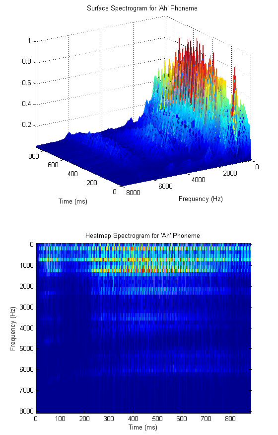
Yet more detailed investigation shows that different phonemes (particularly vowels) have characteristic regions of high energy in the spectrum. These peak regions are called formants, and their locations can be used to extract both phoneme and (at a higher resolution) speaker information. The vowel formants are well studied and their particular locations are available for reference^[6]. Considering again the 'ah' phoneme, the reference indicates that the first and second formants are centered at 700 Hz and 1150 Hz respectively. The audio spectrogram for our recorded 'ah' is shown in the figures below, where we have used a smaller FFT to de-emphasize the fundamental and its harmonics. (A spectrogram is simply a time series of FFTs taken on consecutive blocks of samples. We include both a surface and heatmap below). We see that there is significant energy in the predicted frequency bands.

In order to quantify the amount of energy in the various regions of the spectrum, it would be natural to design a series of overlapping filters that cover the active region of the spectrum. It turns out that this technique is used quite often, and leads us to our primary analysis tool - the mel cepstrum. Consider the triangular filter bank shown below.

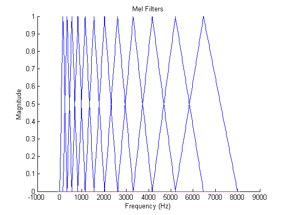
The filters are designed so as to be equally spaced in the mel domain, a logarithmic scale related to frequency by^[7].

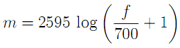
or inversely

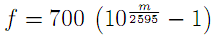
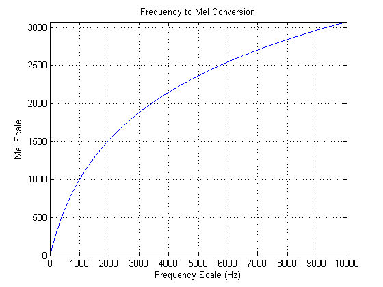
The mel scale mimics the logarithmic perception of pitch as experienced by humans, and is designed such that 0 and 1000 are equal to themselves in both the mel and frequency scale^[7]. This is demonstrated in the plot below, which is simply a graphical representation of the formula above

Once the mel filters have been designed, one can calculate a vector of mel weights for a brief audio sample as the inner product of the audio FFT and the mel filters. The number of mel filters to use is a system parameter, but the literature indicates that 12 is typically sufficient for speaker recognition. The last step that is taken is to compute the discrete cosine transform of the logarithm of the mel weight vector. The resulting vector is called the mel-frequency cepstrum (MFC), and the individual components are the mel-frequency cepstral coefficients (MFCCs)^[8]. It is not completely clear to the authors why this last step is taken, but given that it is commonly used, we decided to implement it. The full process block diagram, then, is given below.

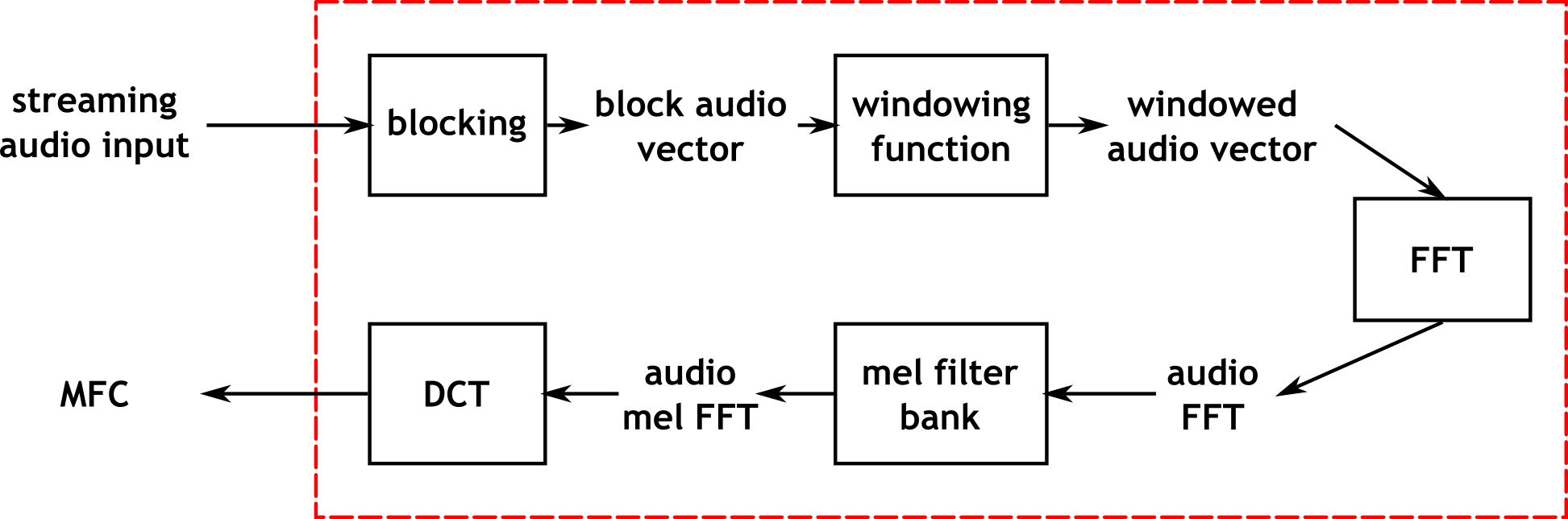
The windowing function referenced in the diagram is typically a Hamming or Hanning window, and is used to reduce smearing of peaks in the frequency domain. The improvement realized by introducing these windows was unclear to the authors, so we implemented them as parameters to the system which could either be used or left out.

Once the MFC has been calculated, the problem of classifying the speaker still remains. Fortunately, the problem is now formulated in the well studied language of machine learning, and the relevant techniques can be applied. Much of our work, then, was in training and evaluating various predictive models, which we will now briefly introduce.

The first (and perhaps simplest) classification method is nearest neighbor search. This technique attempts to classify a vector according to the identity of the nearest point in n-dimensional space, where n here refers to the length of the mel cepstum vector. In the more general case, the k nearest neighbors are found, and classification is based on the plurality winner of the k points. The distance metric used to evaluate nearness of points is typically chosen to be in the class of L^p norms, given by^[9]

where we recognize the L²-norm to be the traditional Euclidean distance. As a caveat when performing nearest-neighbor search, one must be careful to normalize each dimension to prevent large magnitude dimensions from overwhelming smaller magnitude ones. Thus, it is common to compute z-scores for each vector component based on the mean and variance for each dimension.

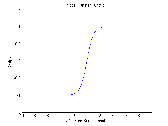
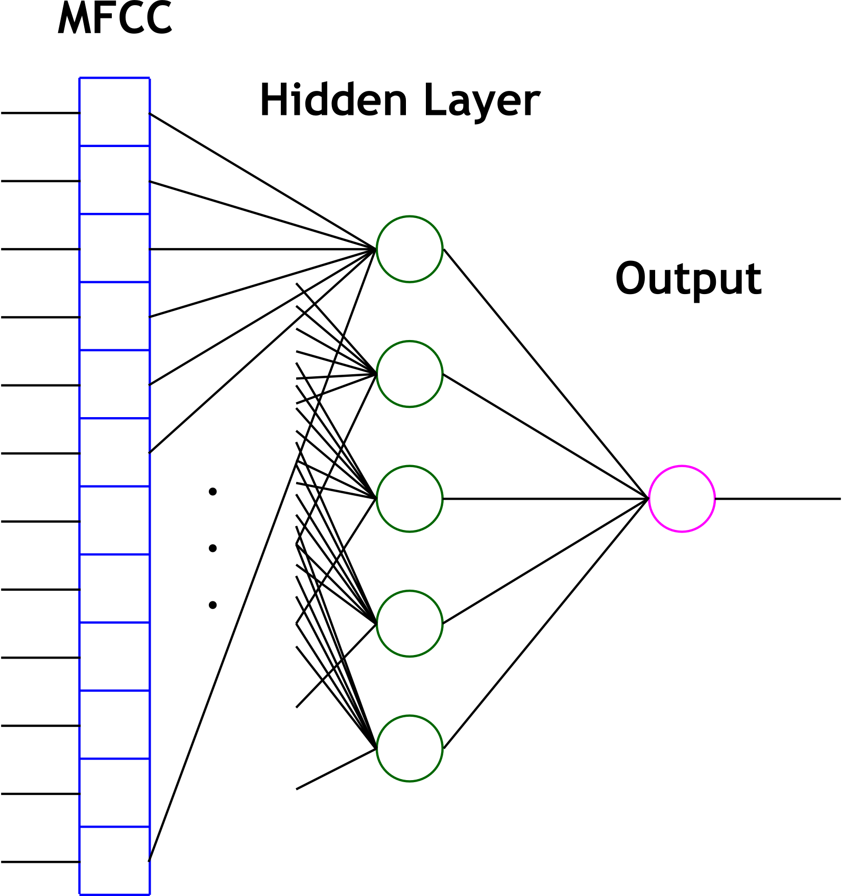
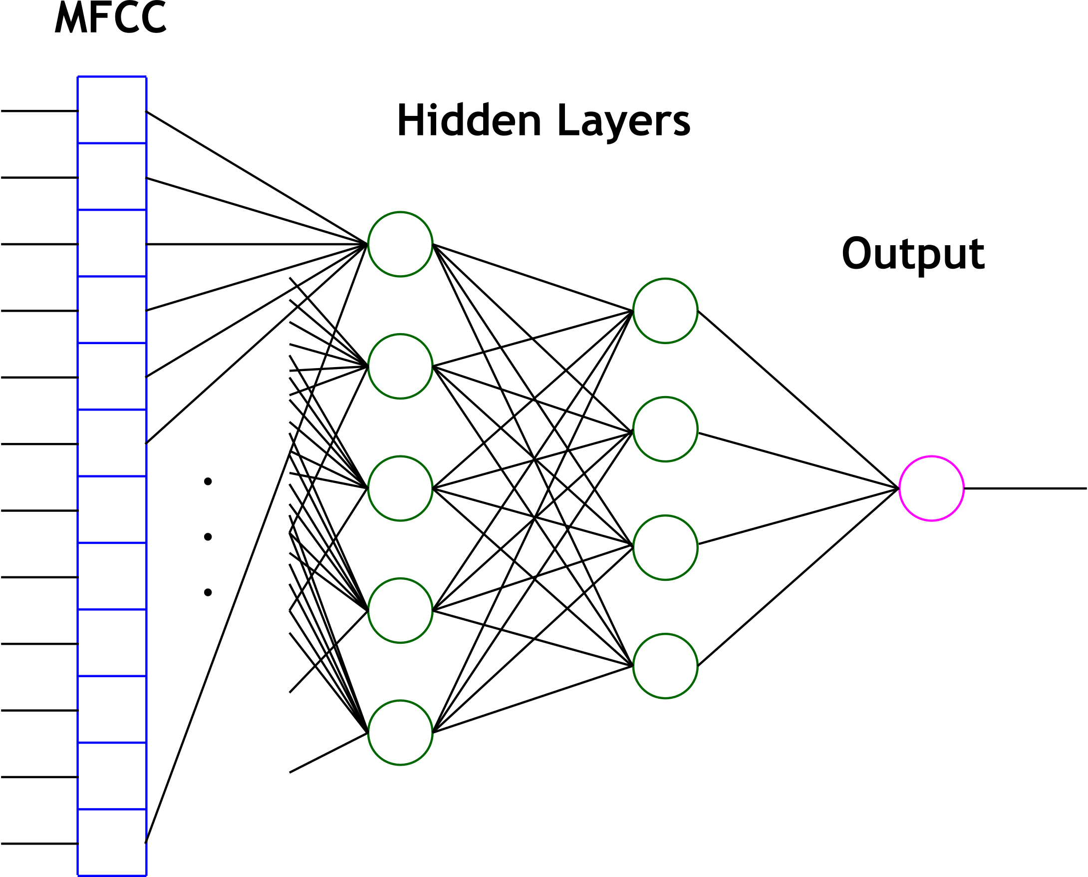
The second primary technique that we used for cepstrum classification is the artificial neural network. The study of neural networks is very large and we will not attempt to introduce it here. Since we wished to run the network in real time, we decided to use one of the simplest neural network variants - the perceptron network. Such a network computes hidden layers of nodes by computing sums of weighted inputs, and then generates an output prediction based on a similar sum of weighted outputs from the hidden nodes. Consider the following canonical node.

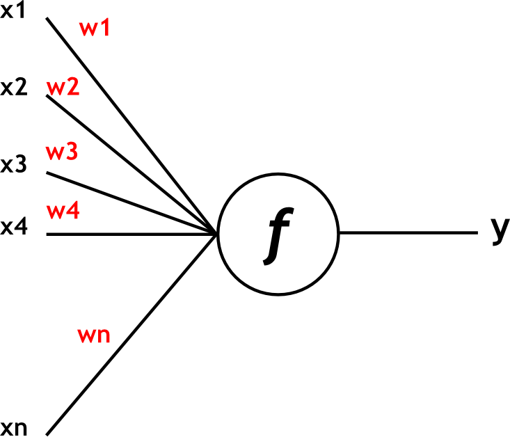
For the perceptron network, the output y is computed as

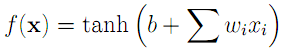
where the x vector is the input, b is the offset bias, and the w vector represents input weights. The hyperbolic tangent, shown below, is used to "tame" outliers, which would otherwise lead to large outputs.

The algorithm which has just been presented is quite complicated, and has many "moving parts". Thus it was expected from the outset that a significant portion of the computation would be done in C on the NIOS II core. However, it is desirable in terms of speed, and more fully utilizes the available hardware, to do processing in Verilog. Conveniently, we discovered that Altera had already writted a fully functional, parameterizable, FFT hardware module. Also available in hardware was a module to control the audio codec, with which the authors were already quite familiar. Thus, in reference to the block diagram presented above, we decided that a natural separation of work would be to perform all steps up to and including the FFT in hardware, and then to compute the remaining steps using the NIOS II processor.

The first step in hardware was to capture and store a sequence of audio samples such that they could be passed to the FFT controller. Capturing samples is a straightforward process which involves communicating with the audio codec. The codec controller was already provided to us and is available in the code listing. The codec registers discussed in the data sheet were configured to meet our particular application requirements, and are summarized below. The most notable changes from the typical setup are the reduced sampling rate of 32kHz (and the corresponding de-emphasis) and the microphone input instead of line input.

Register Num / Name	Value	Notes
R0 / Left Line In	9'b0 0001 1111	High Gain
R1 / Right Line In	9'b0 0001 1111	High Gain
R2 / Left Headphone Out	9'b0 0111 1001	Unity Gain
R3 / Right Headphone Out	9'b0 0111 1001	Unity Gain
R4 / Analog Audio Path	9'b0 0001 0100	Mic->ADC, DAC On, No Bypass or Sidetone
R5 / Digital Audio Path	9'b0 0000 0010	De-Emphasis at 32kHz
R6 / Power Down Control	9'b0 0000 0000	All On
R7 / Digital Audio Format	9'b0 0000 0001	MSB First, Left Justified, Slave Mode
R8 / Sampling Control	9'b0 0001 1010	32kHz, Normal Mode, 384Fs Oversamp
R9 / Active Control	9'b0 0000 0001	Activate

The next step was to store a block sequence of samples such that they could be passed to the FFT controller. We tried several storage methods before settling on one that worked well. The simplest approach here would be to store the samples in registers. But at a sample width of 16 bits, a lengthy block begins to quickly use up logic elements, which is undesirable for a large design. In response to this, we next attempted to use off-chip SRAM. Although this method worked in principle, it became increasingly difficult to arbitrate reading and writing. In addition, SRAM suffers from the inconvenience of setting up write enable and address a cycle before performing data operations. The final approach we settled on, then, was to use dedicated on-chip storage elements via the two-port RAM megafunction. This method enjoys the benefits of both previous methods, without their shortcomings. Specifically, the RAM megafunction handles arbitration, so that the designer can read and write at the same time, but does not use up valuable logic elements.

The next step in the block diagram is to perform windowing on the audio sample block. In our implementation, this step is actually performed as the audio block is being filled, and is thus not a separate step. The weight value applied to the incoming sample is provided by a ROM of precomputed values. The MATLAB script to compute this ROM is provided in the code listing.

Once the windowed audio sample block has been obtained, we must now interface with the FFT megafunction. The bulk of the hardware design is in this interface module. The FFT megafunction data sheet is listed in the references section and discusses the various possible parameterizations of the module. As one would expect, the megafunction allows you to specify the FFT length, bit width, and whether it is a forward or inverse FFT. Of particular interest, the megafunction also allows you to specify one of four implementations, which determine the extent to which you may provide streaming input samples. For example, the "Streaming" data flow architecture allows you to continuously provide input samples, whereas the "Block" architecture requires that you wait for the FFT to complete and the output buffer to be clear before another transform can begin. Fortunately, the interface signals (which adhere to the Avalon ST specifications) remain virtually unchanged between the various architectures. Thus, we wrote the controller before having decided which implementation we would use.

The particulars of the controller design follow from the timing diagram provided in the data sheet, and are not terribly instructive to discuss. The interested reader may find the commented code in the code listing appendix. Suffice it to say that there are two state machines, one for the input samples and one for the output samples, which clock data into and out of the megafunction by asserting the Avalon signals as prescribed by the data sheet. A transform is initiated by filling a RAM with input samples and then signaling the controller to start. When the transform is complete, a done signal is raised and the output samples are available in a two port RAM similar to that used to store the input. As a convenience to the user, the three relevant clock rates (input sample RAM clock, controller state machine clock, and output sample RAM clock) may all be different. Achieving this goal was the source of many frustrations, but the result is pretty rad.

The NIOS II that we used for our application was actually rather simple (though powerful). We employed the largest and most powerful CPU in order that our software classification algorithms would run as quickly as possible. In addition, we phase locked the NIOS to 100 MHz from the base clock of 50 MHz. When parameterizing the CPU, we made sure that it had plenty of instruction and data cache (4KB of each) and we enabled hardware division. We also enabled the hardware floating point multiply and divide. We used a JTAG UART interface and LCD for display during debugging, but they are not used for the final applications. SDRAM was used for storing the program because it is large enough to hold our code base. We were also not sure how much code we would be writing so we thought we would be safe and use the largest memory storage for program memory.

Communication between the CPU and hardware is performed using only parallel I/O (PIO) ports. The first set of PIOs are for the interface with the FFT controller. One bit is required to signal the FFT Controller to begin sampling and applying the FFT transform (this is a single line output PIO called FFTStart). Another bit is driven by the FFT controller and indicates that a transform is complete (this is a single line input PIO called FFTDone). In addition, we need a way to read the transform results from the RAM in the FFT controller (this RAM stores the FFT power spectrum after a transform is complete). We accomplish this using two PIO busses. The first (FFTAddr) is an output bus that specifies the FFT RAM address to read. The address is a number between 0 and 511 (the first half of the 1024 point FFT result) and is thus 9 bits wide. The second (FFTPower) is an input bus that returns the 16 bit value at the specified address in the RAM. Finally, we have a PIO input bus from the FFT controller which returns the exponent associated with last FFT. (The exponent is an output from the FFT megafunction and indicates the overall gain necessary to apply to the tranform in order for it to be the proper magnitude.) The exponent was employed here to detect whether there was anything being spoken (or any noise) by detecting deviations from a silence value of the exponent. For our FFT implementation it is 6 bits wide.

The DE2 user interface (UI) is outlined above. Board signals are communicated with the NIOS via PIOs (excluding reset, which is only used in hardware). Application Mode selection consists of two switches encoded as shown. This is accomplished using a 2 bit PIO bus input named AppSwitches. For nearest neighbor speaker identification we require two additional inputs. First, we need a signal that indicates whether the system is supposed to use the audio input for training or testing. The training/testing signal is implemented using a single line PIO input called Train (negated the signal for positive logic). Second, we need an input to specify the ID of the thing being trained. The ID is a 4 line PIO bus called VowelID. We arbitrarily decided to allow 4 different training "classes" (these could be speakers, vowels, etc). The bus is driven by 4 switches on the DE2 encoded as one-hot. That is, we assume only one switch is enabled at a time during training (to be safe, we also employ a priority encoding scheme in software). We chose 4 adjacent switches so that we could light the LEDs above each one when in identification mode. The final IO is for LED feedback, and consists of a 4 bit PIO output bus (VowelLEDs) for the nearest neighbor identification. We only ever activated one of the bits on this bus to light one of the LEDs above the switches used for training. For the other application modes, we needed a nice way to indicate "accepted" or "not accepted." For instance, to tell whether something spoken is a vowel or not, or whether the person speaking is the training target (in our case Parker). This was done using two PIO single bit output lines, one connected to a green LED (cleverly named GreenLED) and one to a red LED (RedLED). As one would expect, the green LED indicates "accepted" and the red, "not accepted."

The final SOPC builder setup for the NIOS can be seen below.

Interfacing the SOPC with hardware was straighforward and can be seen in the verilog code of DE2_TOP.v below. Essentially, we hooked the PIO as described above, made a 100MHz PLL line for the clock and hooked that up, hooked our reset button up to the active low reset, and hooked all the IO appropriately to our FFT controller. We also had to hook up the SDRAM signals and make sure to phase delay the SDRAM clock by 3ns as described in various documentation.

The code running on the NIOS II executes our algorithms on the raw FFT power spectrum data. The full commented code is presented in the code listing, but we will summarize it here. At the highest level, the code runs in an infinite loop. At the beginning of the loop, an FFT transform is initiated in hardware and the code waits for the signal that it is complete. The waiting is performed by spinning on the PIO FFTDone flag. Once the FFT is complete, we check the FFT exponent to see if appreciable input was recorded on the Mic input line. This tells us whether someone is speaking (although one often has to speak up for it to register). We determined experimentally that the value of the exponent when subjected to silence is 62 (unsigned) and we check whether the unsigned exponent value is less than this to determine if we should continue to the analysis. If we decide that there is only silence on the line, we clear all LED feedback that may be currently active (we don't want feedback if there is silence on the line). If there is a deviation from the silence value, we continue with the body of the processing.

The first step is to load the power spectrum into memory and convert it to floating point (the conversion is not strictly necessary, but was convenient for our analysis since our algorithms were floating point algorithms and we were not too pressed for time). Since we included hardware floating point in our CPU, floating point operations are quick. We use the PIO interface that we created to set up each address (0-511) and then read the value of the spectrum on the data line. We cast this to a short (since it is 16 bits) and then cast to a floating point number storing the result in a floating point array. At this point, we have the power spectrum of the FFT (of something that is non-silence) in memory. Now we can proceed to process it.

We begin our processing by shifting the spectrum to the Mel scale using a call to our "melshift" routine with the current power spectrum and several parameters including the length of the spectrum (512), the destination array to store the shifted spectrum, the number of frequencies to do (the first 12), and the sampling rate with which the samples were taken which were used as input to the FFT (32KHz). The shifting is described in the theory section above and the details of how we accomplished this algorithmically can be seen in the code listing below.

We next compute the discrete cosine transform of these spectral points to obtain the MFCCs using the "dct" funtion, passing a pointer to the Mel shifted power spectrum (the first 12 components anyway), a pointer to an array to store the results, and the number of cepstral coefficients to produce (again 12). As with the shifting, this is described in the theory section above and can be seen in detail in the code listing. The DCT computation is less efficient than other known methods but as we only need 12 points for our particular application, this was considered acceptable. At this point in the code, we have an array of 12 floating point MFCCs. We can now perform the selected application (based on the application mode switches).

The first (0) application is APP_VOWEL_RECOGNITION. This is an application which tries to decide whether the current thing being input through the Mic is a spoken vowel. The first thing this does in the case statement is to clear any LED feedback for another application. This application uses the green and red LEDs for feedback as described in the NIOS II Design section above. Thus we want to clear the LED feedback for the nearest neighbor application. We then call a function "vowelCheck" which determines if the MFCC array respresents a vowel or not and provides the appropriate feedback. Then the program loops to the beginning again. The "vowelCheck" routine is actually rather obscure. We perform the vowel detection using a two layer feed forward neural network that we trained in Matlab using the Neural Network Toolbox's nftool application. The resulting network has the form shown below.

We took the input weights and layer weights from the Matlab structure as well as the input node biases and ouput bias. All of this is stored in memory and can be seen at the top of the program with appropriate commenting ("Neural net for vowels"). We also emulate the transfer function for each node which is a hyperbolic tangent. The routine for the hyperbolic tangent (tanh) is taken from the math.h standard library package. All the vowelCheck function actually does is evaluate the neural net for the input MFCC vector and say yes or no based on an arbitrary cutoff that we specified (a value from the net greater than 0.4 means a vowel, otherwise not). The evaluation of the net is done by first normalizing the array of MFCCs to values in the range of [-1,1]. This is done using the data that we trained on and some helpful coefficients that we generated in matlab for this purpose. The reason this is done is because Matlab's nftool automatically preprocesses training data to be in this range when it is training the network. Thus we needed to do this to have appropriate data for the net to classify. We then weight each input by the input weight and sum them together for each input neuron. Next, we add the bias and apply the transfer function (tanh) on the output of this function to obtain the output of the neurons. For the output of the network we apply the weights of each input neuron to its output and sum all of these together, then add the output bias and apply the transfer function. This is our network output. Then we just check if the output is above 0.4 and ouput a 1 for yes and a 0 for no. We then use this as logic values from the function and do the feedback as described previously.

The second (1) application is APP_VOWEL_IDENTIFICATION. This is a little misleading because it does not have to be vowels, it just seems to work best with them. This application uses three functions which were written to do 1-Nearest-Neighbor machine learning which is discussed in the background section above. The first of these functions is the "initdbase" function which clears all of the previously stored MFCCs and is called at the beginning of the program. Essentially this means we have to reset the system to clear the training samples. We could have chosed to do this a different way, such as when another application was run, but it was decided that this would be more overhead than it was worth. At the beginning of this application's case statement we clear the red/green LED feedback because we are going to use the 4 vowel identification LEDs instead. We then look to see if the training button is being held (this is a PIO input which is high when the fourth button on the DE2 is being pressed). If it is, then we should use the current MFCC array for training the 1NN method. We then look to see what the highest numbered active training ID switch is. If none of them are up, we do nothing. Otherwise, we call the "addtrain" function with the number of the switch (3 for the highest, 0 for the lowest). The "addtrain" function essentially just adds the MFCC array to a database with the associated label (specified by the ID switches) if there is room in the database (there is a maximum number of examples per ID). The function also stores some other values so that normalizing the coefficients and finding the closest "point" will be easier and quicker when we do classification. This code can be seen in full detail in the code listing below if the reader is interested to see exactly what values are calculated and stored during training. Finally, in this application, if the user is not pressing the training button, we try to classify the MFCC array to one of the ID's used in training. This is accomplished by calling the "nearestneighbor" function with the MFCC array. This function does the grunt work of the algorithm. It first normalizes the coefficients by finding the mean, variance, and standard deviation of each coefficient seen so far and then normalizing with these values by taking the difference of each of the values from the mean and dividing by the standard deviation. Once the coefficients are normalized, we then find the normalized trained coefficient array with the lowest "Manhattan Distance" from the provided MFCC array. We then return the label on this MFCC array as the label to the provided example. The details of the implementation of the algorithm to find the trained MFCC array with minimum distance can be seen in the code listing below. This algorithm is called 1 Nearest Neighbor because it classifies a new example with the same label as its one nearest neighbor.

The third (2) application is APP_SPEAKER_VERIFICATION. This is our attempt at verifying a speaker. We used Parker as the speaker to be verified and trained a three layer feed forward neural network in Matlab in the same manner as the vowel recognition network (but with a slightly different tool - nntool instead of nftool). This network, shown below, has 5 input neurons, 4 inner neurons, and one output neuron.

After testing with this network, we realized that it was not performing well and had to replace it. In order to improve our results, we decided to build a larger data set of speech samples. Jordan and I each spoke for 10-15 minutes generating hundreds of samples representing positive and negative examples of "Parker" speech. We then trained a simpler network but with more input nodes (20 input nodes) which has the same structure as the one for identifying vowels. We put the network into the code in place of the three layer network described above.

We trained the network on only MFCC arrays that pass the vowel recognition test. We noticed through our testing that vowels seem to work best for classification. Sounds like "sh" and plosives have rather undefined and noisy spectrums. After training the network, we put the weights, biases, and necessary constants into Matlab as before and made a function "classify" which evaluated the network. Additionally, the output was deemed to indicate a positive "Parker" verification when it was above 0.9. The code in the case statement for this application simply clears the nearest neighbor feedback as does the vowel recognition application and then calls this method on the MFCC array, and then if it sees a 1, lights the green (verified) LED, and otherwise lights the red LED.

Finally, we added an application (3) which combines the one nearest neighbor approach and the neural network in order to get a better verification result. Essentially what it does is call the classify method on the current MFCC array. If the classification neural network says that it is Parker, we ask the nearestneighbor method whether the MFCC array's nearest neighbor has an ID of zero. This means that this application is intended to be used as follows: train ID 0 as Parker and then ID 1, 2, and 3 with other people, then use the application as if it is the same as the verification application above. This application has the same LED feedback as the verification application and has the same training interface as the vowel identification application.

Additionally, we found it useful throughout debugging to have the program print out various values and arrays of coefficients so our code is littered with debugging code. This code however is encompassed in preprocessor directives and is only included for certain debugging levels defined at the top of our code. Thus for non-debugging versions, we set the DEBUG define to 0, and none of this code is actually compiled in (and thus not executed).

The results for the vowel recognition application mode are summarized in the table below. Each of the authors uttered the phonemes in the first column several times (or for a reasonable duration), and the classification results are given in the body columns.

	Jordan		Parker		Total
Phoneme	Not Vowel	Vowel	Not Vowel	Vowel	Not Vowel	Vowel
AH	3	13	1	16	12%	88%
EE	6	12	12	7	49%	51%
OO	11	6	2	18	35%	65%
OH	4	12	0	19	11%	89%
II	3	12	10	9	38%	62%
UH	12	4	8	16	50%	50%
SH	12	0	18	0	100%	0%
TT	13	0	13	0	100%	0%
KK	14	0	8	0	100%	0%
MM	19	0	18	3	93%	8%
NN	13	1	11	6	77%	23%
ZZ	15	0	14	0	100%	0%

The truth table is easily computed and is shown below. We can see that the false positive rate is kept very low, as was desired, while keeping the true positive to true negative ratio at a healthy 2:1.

	Act. Vowel	Act. Not Vowel
Pred. Vowel	144	10
Pred. Not Vowel	72	168

The results can be seen in the two tables above. Basically, it was fairly successful on the consonants and vowels with which we trained the neural net and slightly less successful on those that we didn't such as "uh." Also, the vowel "ee" seemed to prove difficult for our vowel recognizer. Essentially, what we took away from this part of the project was a tool which helped us to find vowels. The vowel recognizer was very good at not saying a non-vowel was a vowel which meant we could rely on it to pass mostly vowels. Since we used this in other parts of the project to filter vowels out of speech, this was very good. We could then assume that most of the MFCC arrays that were classified as vowels were in fact vowels and could be treated as such for further analysis.

The results for the vowel identification application mode are summarized in the misclassification matrix below. The nearest neighbor database was trained on only one of the authors voices (Jordan's) but was tested on both authors. The results are nearly perfect for both authors.

	Act. AH	Act. OH	Act. OO	Act. EE
Pred AH	24	0	0	0
Pred OH	0	39	0	0
Pred OO	0	0	29	3
Pred EE	0	0	2	22

This application was the most successful of all of our applications. The table above speaks for itself. We do not know for sure why it performs so well other than to say that there are probably very disctinct differences between vowels in terms of frequency spectrum analysis. The nearest neighbor algorithm was able to pick up on these differences with very few points of training data.

The graph above shows a comparison between the false positive and true positive rate of the neural network speaker classification. Many of the results of the scheme can be extracted from this chart. The method proved promising, as the number of false positives was quite low in comparison with the number of true positives at any given level of cutoff for the classification (based on the value output from the verification neural network). As we said before, we used 0.9 as our cutoff, but this was a rather arbitrary choice. One good thing about this cutoff is that there is a fairly low false positive rate which is what we wanted. The technique was not perfect however and there were many false negatives. Throughout the verification development, we were committed to the idea that, in a recognition system, false positives are much worse than false negatives (although we can imagine in something like a phone banking system having to say the same pass phrase over and over again could be very annoying).

In an attempt to improve the false positive rate of our speaker verification system, we used a fourth application which combined the one nearest neighbor approach with the neural network for speaker verification (of Parker). The application is described above. The result of one of our runs with this system was a true positive rate of 34/143 samples of Parker speech or 24% and a false positive rate of 16/143 samples of Jordan's speech or 11%.

We experienced mixed success with our various experiments. On the one hand, the vowel tests appear to work very well, especially the vowel identification. This may be due to the small database of vowels being used, but we expect that if extended to encompase futher phonemes, the performance would not suffer terribly. On the other hand, the speaker identification/recognition experiments performed poorly in general. This might be casually attributed to the inherent difficulty of the task. After all, humans still occasionally make mistakes when faced with this task, and we are highly evolved to handle it. But this is a rather unsatisfactory conclusion. We may propose some more specific reasons. For instance, the speaker identification application is built on top of the vowel recognition application, and thus suffers from any problems of this base task. It is also possible that we are not using the appropriate number of cepstral coefficients, or that the filters do not cover the optimal region of the spectrum. These are experiments that could have been performed given more time. Finally, it is possible that the underlying FFT length and audio sampling rate are not conducive to capturing the best periods of speech. We did however experience what we would deem modest success in this persuit and also were able to make some interesting applications to perform related functions like vowel recognition and identification.

Given more time, we would have liked to persue more of our suspicions about what was causing our poor performance. In addition, we would have liked to try more machine learning techniques. Specifically, Hidden Markov Models (HMMs) and Support Vector Machines (SVMs) may have performed well on this problem. Also, dynamic neural networks with feedback and time delay would have been very interesting to work with. It seems that they are used in many related problems where time varying patterns are classified and it would have been fun to attempt an implementation in software or hardware for this particular application. If we could build a library of such techniques, it is also possible that the problem would have cracked when subjected to a medley of solutions. As a final note, we would have liked to implement our own version of neural network training instead of relying on MATLABs training (whose implementation specifics we are still unsure of).

We feel that the project was a success in terms of the knowledge and experienced gained as well as some noteworthy results. While our results did not necessarily live up to our expectations at the outset of the project, we are happy with what we have accomplished. We are confident that were we to begin a speech processing project in the future, we would be much better prepared.

[1]Wikipedia: Airstream Mechanism
[2]Wikipedia: Phonation
[3]Wikipedia: Larynx
[4]Wikipedia: Human Voice
[5]Wikipedia: Vocal Folds
[6]Wikipedia: Formant
[7]Wikipedia: Mel Scale
[8]Wikipedia: Mel Frequency Cepstral Coefficient
[9]Wikipedia: Lp Space

Audio Codec
FFT Megafunction

Ganchev et al. Comparative Evaluation of Various MFCC Implementations on the Speaker Verification Task.

Hasan et al. Speaker Identification using Mel Frequency Cepstral Coefficients.

Sigurdsson et al. Mel Frequency Cepstral Coefficients: An Evaluation of Robustness of MP3 Encoded Music.

Task	Performed By
FFT Controller Hardware Design	Jordan
Interfacing of FFT Controller with NIOS	Jordan and Parker
NIOS Design and UI	Parker
Research	Jordan and Parker
Data capture and Neural Network Training	Jordan and Parker
C Application Development and Algorithm Design	Jordan and Parker
Website	Jordan and Parker

Bruce Land - Infinite knowledge and helpful guidance

Terasic Technologies - Codec Controller Verilog Module and helpful Examples, DE2

Altera Corporation - FPGA, Code Examples, DE2, IP (FFT and RAM modules), Quartus and NIOS II IDE

Alhassan Mohamed Fattin (Teaching Assistant at Cairo University) - Effort in helping us attempt to improve the interface between the FFT and the NIOS