
For our final project, we implemented hardware to create fractal landscapes on the FPGA, displaying on the VGA. Fractal landscapes are procedurally generated landscapes, calculated fractally with a degree of randomness to make them look very natural. We believed this would be a good utilization of the FPGA due to the massive potential for parallelization. We started by simulating the algorithm in MATLAB to get an understanding of the process, then moved to the FPGA. To get the largest landscape possible, we parallelized the algorithm in one direction and serialized in the other for a good balance of speed and hardware utilization. We then exported the result to the VGA screen for visualization, and compared the speed result to the HPS implementation. In the end, we could generate 65x65 landscapes around 4000 times faster than the HPS.
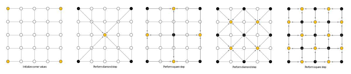
Fractal landscapes utilize a simple algorithm to generate beautiful, natural looking landscapes with a degree of randomness. Each point is just the average of the surrounding points in a given square, with an added degree of randomness. The major restriction on the system is that it must use (2N+1)x(2N+1) sized grids, such that each step of the process can break the landscape up into progressively smaller, equal sized squares that themselves are (2N+1)x(2N+1) sized grids, where N decreases with each step. To start with, the four corners of the landscape are initialized to set the general shape of the landscape. However, even with all corners initialized to zero, the landscape will still have distinctive features. First is the diamond step of the algorithm, with the square size being the entire landscape, and calculates the center point. Next is the square step, still using the entire landscape, and each center of the edges is calculated. The landscape is then broken up into four even squares, and the process is repeated. The landscape continues to be broken down into smaller squares until the entire landscape is full, which takes N steps. This process can be seen below in figure 1
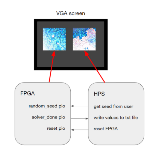
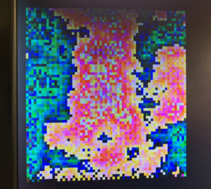
As seen in figure 2, the HPS and FPGA independently calculate the height values for a fractal landscape after being reset with a user-inputted seed. The HPS communicates this random seed to the FPGA through a PIO port. The FPGA indicates it is finished with the fractal landscape calculation also through a PIO port. With this done indicator, the HPS is able to time both its own calculation and the FPGA’s calculation so we can compare their speeds. The FPGA writes directly to the left-half of the screen through VGA SRAM, while the HPS writes to the right-half of the screen also through VGA SRAM.
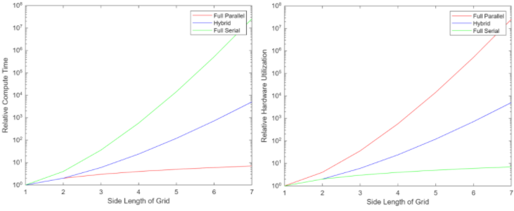
We spent a lot of time considering the best way to implement the algorithm on the FPGA. We wrote our first implementation in MATLAB, which was extremely useful for seeing how the algorithm functions in general. However, the method was completely iterative, visiting the correct points one at a time to calculate their values. Each point is only visited once and (with no optimization) requires the value of four other points to be calculated. This means that our compute time scaled linearly with the number of points in the grid, or scaled as the square of the side length of the grid. Of course, this MATLAB implementation was a relatively “naive” approach in that it was fully iterative: since the diamond square algorithm has a fractal-like nature, there was an opportunity for immense parallelization.
To think about how this parallelization might take place, we created a series of images that represented which points were already known at each step of the algorithm, and which points needed to be calculated in that step.

One of the first decisions we had to make was the fixed point structure of our data. The more granularity we had, the better the landscape would look. However, the smaller the data, the more point and logic we could fit on the FPGA. Initially we believed that by using a 10 bit structure, we could use a 513x513 grid utilizing 256 M10K blocks each with 1024 entries, plus registers for the extra row and column. However, due to large logic utilization that did not end up being possible. We still had all of our logic in 10 bit for the majority of the project, until we realized that our logic was not fitting on the board. At that point, we moved to 8 bit logic, as that would utilize only two ALMs per data point rather than three. This had the added benefit of directly translating to the VGA screen, because the color value is also 8 bit.
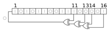
In order to implement the required randomness for natural landscapes, we utilized a linear feedback shift register (LFSR) module. This simple module produces a series of pseudo-random numbers by starting with a seed and repeatedly shifting and XORing the result. Each cycle, this LFSR was queried for a new random number for each column.
Once the entirely parallelized version of our algorithm was confirmed with Modelsim testing, we moved on to a more practical implementation for the FPGA. Because we would eventually be moving to M10K memory storage, we could not read every pixel across the board at once for calculations simultaneously. Therefore, we theorized a way to most efficiently traverse the entire map while only doing a single M10K read per cycle. Our resulting algorithm was similar to that used in the Lab 2 drum solver, where we serialized rows and parallelized columns.
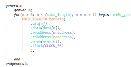
Once the state machine was set up to be accessible for M10K, we set about implementing the memory itself. First, we initialized the M10K to be the appropriate bit width and length, creating them in a generate block, one for each column
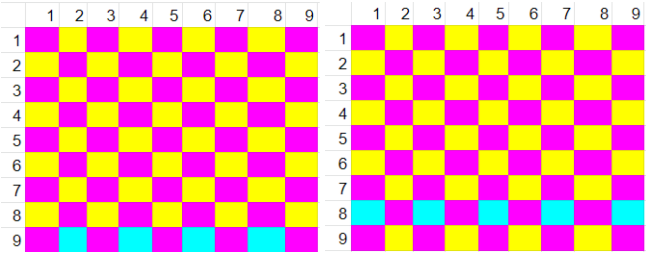
In order to visualize our results on the VGA, we waited until the FPGA state machine was finished solving, which was checked with a done_signal. The signal checked if every row of the last iteration of the diamond-squares algorithm was complete, at which point it would set a flag. Once the VGA state machine recognized this flag, it looped through each point in the M10K block storing the height values and graphed them to the VGA. When we first did this, it looked rather small, so we ended up graphing each pixel twice horizontally and vertically to enlarge the image for easier visualization. To do this, we had an x counter and y counter that would toggle, which we would add to the pixel location on the VGA, resulting in each point in the heightmap taking up 4 pixels on the VGA. There was a corresponding state machine in the read address function that would keep up with this traversal.
The HPS algorithm is purely sequential, so we were able to base the HPS code off of the MATLAB code we wrote to develop the diamond squares algorithm. The HPS uses the #define keyword to alias N and the grid’s side length in its calculation. Then it runs a loop N number of times that calls the do_diamond and do_square functions which populate a 2D array representing the terrain. Each value in the array corresponds to the terrain’s height at that location. Each iteration increases the number of calculations required to complete the computation at that iteration, since each iteration has an increased number of points to solve for. As described previously, the diamond step calculates the height for the midpoint of each square in the current iteration by taking the average of the square’s corner point heights and adding a random number. The square step calculates the height for the midpoint of each diamond in the current iteration by taking the average of the diamond’s corner point heights and adding a random number.
Initially the HPS calculations were overflowing so we had to reorder how the average was calculated to prevent overflow. Our original order of operations was (a + b + c + d)/4 + random. To prevent overflow while still preserving resolution, our final order of operations is (a/2 + b/2)/2)+ (c/2 + d/2)/2 + random. To generate a random number, we use the C standard library function srand(int seed) to seed the RNG with the seed specified, and then call the C standard library function rand(). To bound the random number to fit within range of a signed 8 bit integer, we modulo the result of rand() by 255 (which is 127-(-128)) and subtract 128.
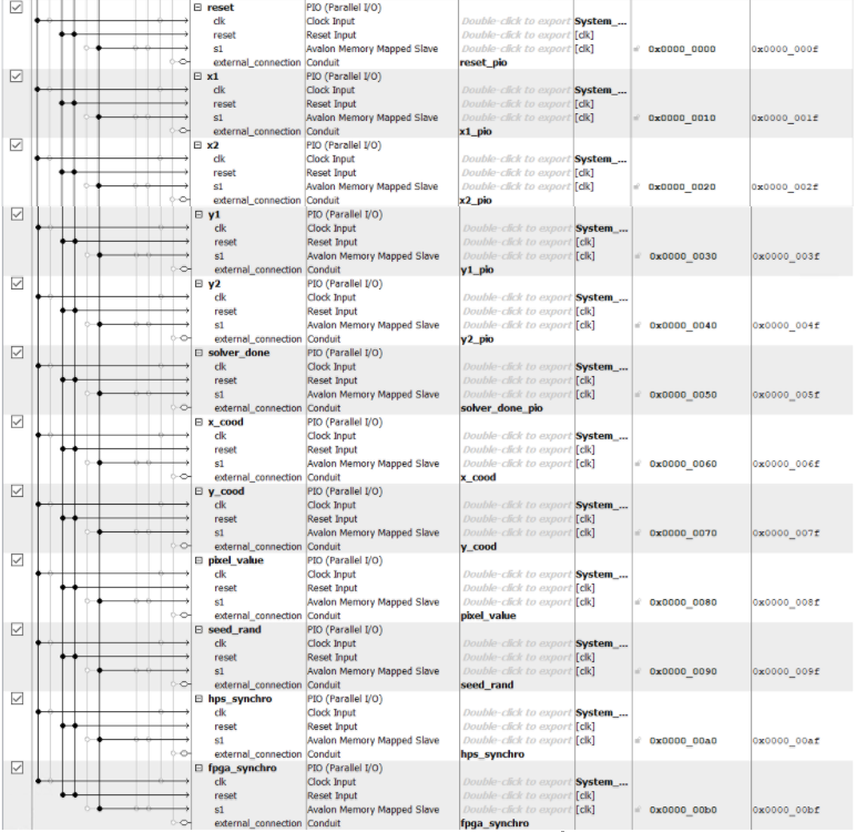
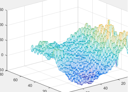
In our Qsys layout (figure 10), we have 12 PIO ports defined but we actually only use 3. We actively use the reset, solver_done, and seed_rand PIO ports to reset the FPGA, indicate the FPGA is done solving, and randomly seed the FPGA LFSRs, respectively. The other PIO ports were created in case we would need them since FPGA compilation takes so long. The x1, x2, y1, and y2 PIO ports were created to randomize the four corner values the diamond squares algorithm starts with, but we decided to hard code the four corners and instead just rely on a random seed to generate different landscapes. The x_cood, y_cood, pixel_color, fpga_synchro, and hps_synchro PIO ports were created to coordinate the solver’s output to the HPS, but we remembered we could just read from SRAM to accomplish the same thing. After the FPGA is finished with its calculations and has written to the VGA screen, the HPS will read the VGA SRAM to copy these values to a text file so we can visualize the terrain in 3D using MATLAB.
To time how long it took the HPS and FPGA to calculate the same size terrain using the diamond squares algorithm, we used the same method as in previous labs. We first record the time at the start of the computation and then record the time at the end of the computation and take the difference to get the time it took for the computation. The computation for the FPGA starts right after reset (reset goes high after being held low), and ends when the value at the solver_done pio goes high. For the HPS, the start of the computation occurs after the terrain map is initialized right before the main iteration loop. The end of the computation is after the iteration loop. Our timing omits the time it takes to write to the VGA screen for both the FPGA and HPS since writing to the FPGA is a bottleneck for both devices and doesn’t give us an accurate comparison of the FPGA and HPS speeds.
Initially, once we loaded the design onto the FPGA, it would stay static. We thought it would be more interesting to quickly generate new landscapes, so we added a PIO port that would seed the FPGA LFSRs and HPS srand() with a user input, creating new landscapes for each input. The interesting part about it being associated with the user input, and not other options like say, the time passed, was that landscapes could be regenerated with the same seed if they were particularly interesting. The seed for the LFSR was then the LFSR index, based on the column, shifted up a bit and summed with the user input seed value. This resulted in us being
Of course, every time we changed the seed, we also wanted to reset the state machine such that it would start calculating again. The reset function was tied to the reset PIO port in QSys, which would simply pull the wire low for a moment while the system reset. This function was triggered each time a new seed was input on the console.
To start with, we wrote our design in MATLAB. This was quite difficult, because although we understood the concept of the algorithm, writing it was quite different. We developed a spreadsheet that would walk through each step of sequentially larger designs to infer how to generalize for any size design. We created relevant variables such as boxSize, the size of a box in a given iteration based on the overall size of the design, and Delta, the distance from a corner of the box that a given point would be. We found generalized equations for these variables as well as how to step through them sequentially, which translated quite well to the FPGA.
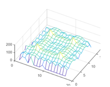
Next, we moved our design to Verilog in ModelSim. We first worked on implementing the LFSR module. We found that early on, the LFSR random values would be quite small in magnitude, and given that our design only took a few cycles to calculate, we never got much variation. To fix this issue, we seeded the LFSR with a higher value, which resulted in immediately larger magnitudes for the random values and a more attractive variation in the landscape. To view these early, small landscapes, we exported the data from the ModelSim simulations into MATLAB and ran a mesh visualiser.
Next, we worked on the algorithm itself. We initially only ran into small, off by one issues as we moved from Matlab, a one-indexed language, to Verilog, a zero-indexed (correct) language. One early issue we discovered was that when parallelizing every step of a given diamond or square step, the same random value was presented for each, resulting in very man-made looking structures
Once we put the design onto the FPGA, we ran into some issues. The algorithm changes the number of calculations required for each step depending on iteration number. This means that the loops we were originally using had a variable iterator, meaning that the number the iterator variable incremented by changed size in each iteration. This is not deterministic at compile-time, so we ran into issues implementing this on actual hardware even though it passed in Modelsim. To fix this, we created a huge conditional statement based on the iteration number. Each iteration number has a deterministic number of iterations, so we were able to get a design to compile by refactoring the code to have a different iterator loop (with a fixed size increment) for each iteration number.
Our code worked when side_length and N were small. As we tried to increase these parameters we ran into a lot of problems getting our design to fit on the FPGA. We kept running out of ALM’s. Our designs did not scale linearly with size; when we tried N = 6 iterations, our design would need to use over 300% of the available ALMs. In addition to the giant conditional statement based on iteration number, we had an even larger conditional statement wrapping this to check if we were in the diamond step, square step, or iteration parameter calculation step (because some parameters changed in each iteration like the number of sub-boxes we needed to calculate values for, and the length of each of these boxes). We also had smaller conditional statements inside each step’s iteration because each iteration number required multiple steps to calculate. All of this to say that we had a ton of unnecessary logic that kept our code compact, which is a result of us having translated the sequential code we developed in MATLAB into hardware as closely as possible to decrease the number of bugs introduced in this transition.
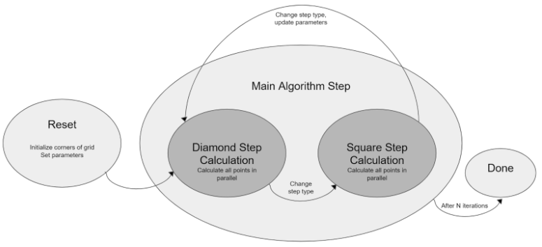
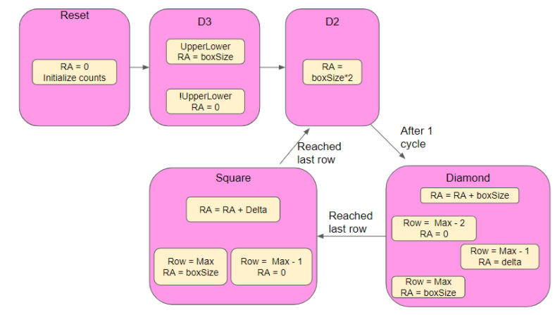
To combat this, we refactored our code and “unfolded” it by making it less compact. Because we know the exact order that the computation will take we were able to make a state machine that has 8 states per iteration number and is pretty straightforward to scale (linear with iteration number). Each diamond step repeats the same state until all the squares have been calculated, and each square step toggles between 2 states depending on the row type to calculate all the diamonds in the terrain. There are some intermediate states that are used to set each step up by loading values from M10K into registers, and recalculating parameters. The state machine contains several registers that we previously conditioned on even though it is no longer dependent on their values. This is because the M10K read address generator module does use those register values, and we wanted to make sure our addresses still worked without disruption. So those registers are still updated as they previously were before transitioning to a state machine.
With this state machine, we were able to fit our design (N = 6) onto the FPGA using the available resources, but we ran into problems with routing. We fixed this by turning on aggressive routing and changing our seed from 420 to 69.
As always, implementing M10K was not within its issues. Due to the modular way we were implementing our code, at first we were having a lot of difficulty getting the right number of cycles for read addresses before they needed to be ready to read. To fix this confusion, we created a separate state machine in a read address module, whose only job was to produce the correct read and write address for each cycle.
We also ran into difficulty with the write enable. During our previous usage of M10K, we never needed to toggle the write enable, because bad data was never being written to the wrong place. However, in this implementation, during our square steps, the column being written would switch off on every cycle. Therefore, we needed to switch off the write enable every cycle, or the data from the previous cycle would write over previously calculated values and produce a blocky, incorrect landscape.
When we finally exported our data to the VGA screen, we did not see anything initially. We ran all relevant variables in SignalTap to find the issue, but the data being written to the pixels appeared valid. Next, we tried simply adding an offset to the drawing indices, which fixed the issue. We believe the screen was not properly calibrated and was trying to draw off-screen.
The final size we were able to achieve was a terrain with side_length = 65, corresponding to 6 iterations required in the diamond-squares algorithm. The chip planner can be seen in figure 15 and took around 2 hours to compile.

The FPGA is much, much faster than the HPS. Using the method described in the timing subsection of the software design section, we found that the FPGA takes approximately 5 us to calculate the heightmap that has side length = 65. For an equally sized heightmap, the HPS takes between 17300 us and 20000 us to calculate. This means that the FPGA can achieve up to a 4000x speed up compared to the HPS.
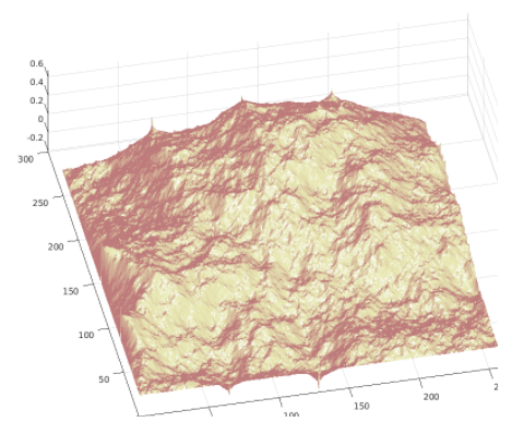
Overall, our design was successful. Our logic ended up being far larger than we expected, and we had to settle for N = 6 rather than N = 9. However, this design allowed us to view both the HPS and FPGA calculated landscapes, which was an unexpected bonus. We also would have liked to visualize our design in 3D directly on the FPGA via the VGA, but due to running into so many issues with space constraints, we did not have time to implement this. Exporting to MATLAB to visualize was almost instantaneous though once we created the script to automate it, so we still got to view all of our designs.
Although we drew inspiration from others’ work, in the end the only thing in common with their designs was the general idea of the diamond-squares algorithm, which is not and cannot be patented.
In conclusion, we were very pleased with the results of the project and our utilization of the parallel hardware the FPGA has to offer.
The group approves this report for inclusion on the course website. The group approves the video for inclusion on the course youtube channel.
Group responsibilities
Nicole: Nicole helped with the diamond squares algorithm development, hps code timing and vga display of algorithm results, refactored code in state machine to meet timing constraints
Alex: Alex helped with the initial MATLAB code and the development of the parallelized and hybrid versions of the algorithm for use on the FPGA. Also helped to write the early versions of the state machines
Katie: Katie was responsible for helping fix the initial matlab code, implementing the verilog code with the rest of the team, creating the M10K module, setting up the random pio hps code, and creating the script to export the data to matlab on the lab computer
FPGA Code
HPS Code
MATLAB Code