F1 Tire Prediction

Sujith Naapa Ramesh (sn438), Felipe Shiwa (fs383), Rishi Singhal (rs872)
12/21/2020
Sujith Naapa Ramesh (sn438), Felipe Shiwa (fs383), Rishi Singhal (rs872)
12/21/2020
In Formula 1 racing, managing tire conditions and race strategies play a vital role in the success of teams during a race weekend. With different tire compounds of choice that vary in expected durability and speed at each weekend, teams must plan how they will utilize the different tire compounds to be the quickest they can. This can lead to differences between one-stop pit strategies, where drivers utilize only two sets of tires as required by the Formula 1 racing regulations, and two-stop pit strategies, where drivers push harder on each tire set but stop and utilize an additional set of tires. Being able to bring the most out of the tire compounds is important for gaining these precious seconds from strategy alone, thus it is important for teams to track the condition of their tires throughout the race.
To attempt to aid this problem, we decided for this project to design and develop a tire degradation neural network model for Formula 1 teams to be able to evaluate tire conditions during a race for all drivers when considering race strategy. We first decided to develop and train the neural network model in Python by utilizing PyTorch, and then created an analogous model within an FPGA. We took this approach since it would be useful if such a model in the future could be integrated into the racing car and provide real-time feedback. For our project, we made some compromises to our design to complete it with our available resources and time, resulting in a simplified model. This model, based on various parameters, approximates the expected impact of a lap on the tire condition to gauge how long the tires will last. This would be clearly useful to teams as they will be able to gauge whether the driver should push harder on the tires for improved performance because they have the tire life to spend, or whether they need to conserve the tires for the sake of the race strategy.
When we first came up with the concept for the project, we considered this as a device that would generate predictions on the tire condition or tire performance on Formula 1 cars based on telemetry data. This would include data such as car acceleration, steering input, brake and throttle traces, among other data points streamed in while the car runs around the track. The device, whether directly on the car or at the pit wall where the telemetry information is received by the team, would evaluate the performance of the tire in real time. Being able to create such models and obtain relevant results during a race would be of significant importance for teams when considering their pit strategy. Teams are able to make projections on how long they expect different tire compounds to last during a race based on the specifications provided by Pirelli for the tires available in a given race weekend and analyzing change in lap time across multiple laps in the practice sessions leading up to the race. However, variable factors such as track temperatures, driver errors, debris, and driving style significantly change the performance of a tire throughout a stint (length of race driven before a pit stop to change tires). While the hope would be for the device to be able to accurately estimate the performance of the tires at any given point in the race, the expectation would be that the device would be one additional factor to consider when adjusting the pit strategy as the race unfolds.
To drive a device to estimate tire performance, we wanted to create a neural network model to approximate the tire performance. To create a neural network model for this problem, multiple factors would have to be considered based on the incoming data and the previous data. Another difficult property to pinpoint would be modeling the effective performance of the tires dynamically for the purposes of training the model. Driver lap times are subject to variability along with track conditions such as a “rubbering in” effect as more laps are driven around a track. Additionally, one of the main problems teams must be concerned with when considering tire performance is blistering of the rubber (small chunks breaking away from the tire as a result of overheating) and flat spots on the tire as a result of locking up the tires under braking. While both cases affect the performance and durability of the tire, gauging a numerical value associated with the impact on the performance of the tire is difficult.
For the purpose of this project, attempting a highly complex network would be impractical since the main premise of our project is to present a method for running neural networks on FPGAs efficiently using the ability of the FPGA to parallelize a large portion of the execution. Furthermore, we do not have access to any telemetry data since teams do not make these accessible since they can provide significant insight into a team’s car performance. Instead, we will simplify the problem and make several assumptions which affect the predictions of our model. However, we are okay with this since the problem is primarily a framing for what we want to demonstrate.
Neural networks are a machine learning method for attempting to learn how to predict an output based on a series of linear functions with associated parameters which can be learned based on training examples. We can better understand how this works by looking at a simple example of a feed-forward neural network, which will be the type of model utilized for this project.
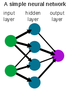
A neural network will consist of multiple layers: an input layer, an output layer, and one or more hidden layers. Each layer consists of nodes where values are evaluated and accumulated. For the input layer, the nodes will consist of the input values provided for the neural network. For the hidden and output layers, the value at the node is a result of a linear function on the values of the nodes from the previous layer. Consider the following image for a single node.
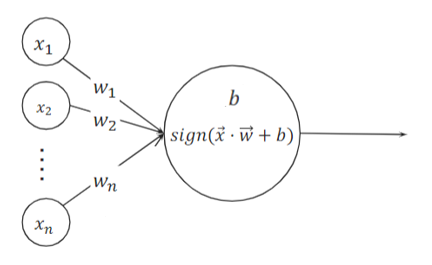
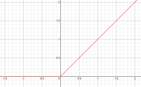
Hidden layers of the neural network additionally tend to have activation functions associated with the nodes. Activation functions are an additional operation on the previous sum to obtain the final value at the node. In the case of Figure 2, we can see in the image that a sign activation function is utilized at this layer. Based on the previously calculated value, the sign function would return a 1 if the value was positive and 0 otherwise. This type of activation function would likely be utilized in a binary classification problem at the output node. Another type of activation function commonly utilized is a ReLU function, as shown in Figure 3. These activation functions are often used to capture more complex behavior of equations with the neural network layout.
We decided to implement a fully-connected, feed-forward neural network similar to the one shown in the image above but with two hidden layers to demonstrate how we can make use of the parallelization potential of the FPGA to perform the evaluation of inputs compared to a traditional processor architecture. To have the model predict the desired labels, the model must be trained by calibrating the parameters of the neural network. Specifically for a fully-connected neural network, the parameters that we are able to train are the weights wi and bias values b previously mentioned. We will go into more detail into how these parameters are trained when discussing training the model. However, we must also consider the features that our neural network will utilize as inputs to make our desired predictions.
There are two main concerns that we must deal with when selecting our features that we will utilize for our neural network. The first concern that we found ourselves faced with is the available information relevant to the calculations we want to make. As previously mentioned, the original concept was to dynamically evaluate tire performance based on telemetry data. However, we do not have access to such data and tuning our design to work with telemetry data may have been significantly more challenging given our timeframe for developing the project. Therefore, we decided to simplify the problem and attempt to make predictions on the effective reduction in tire "condition" after each lap around a track. Since we cannot quantitatively gauge when a tire is too worn out and at risk of giving out and exploding, we will instead attempt to approximate the timing for when the tire condition is less than desirable and resulting in reduced performance such that the driver should pit for a new set of tires.
As far as information we are able to collect, we were able to find the lap times for each of the drivers in a given race. This also included the laps on which drivers had entered the pit lane to change tires. Further, we can obtain the information of which tire drivers are using for each lap from the race broadcasts along with the weather throughout the race. We decided to utilize a single model for all of the tracks instead of making track-specific models, therefore we can also utilize the track layouts in order to define some features we utilize on our neural network.
The second concern that we must generally deal with when selecting our features is the selection and pre-processing of features. The selection of features is important for designing a good model because not all possible features may be relevant for the prediction we want at the output and in fact they may act as confounding variables. Further, if we provide too many features to the neural network then the increased complexity is likely to cause the trained neural network to overfit the training data and have high generalization error when applied to unseen examples. After having selected the features utilized, the representation of each of the features must also be considered. One of the primary concerns when pre-processing features is ensuring that the various features are of similar magnitude when combining them together. This becomes important during the learning process as disproportionate scales in the features will later affect the gradients necessary for the training process during backpropagation.
Since we only have a few features we were able to collect data for, we decided to utilize all of the features that we have collected. Specifically, we utilize lap times, track features, current tire compound in the form of expected tire life, and weather. For the lap times, we decided to normalize the lap times and expected tire life for each race. The tire life is normalized based on the different compounds available rather than all of the existing inputs since repeated instances of tires are not important for considering them as different feature values. For the track features, we represented them as three separate features with each containing the number of slow speed, medium speed, and fast speed corners respectively. For the rain value, we just use a 1/-1 indicator as to whether it was raining for a given lap.
We mentioned earlier that there is the issue of numerically evaluating tire degradation, both as the current tire degradation and as the change in tire condition, and that instead we will create the model to evaluate when the tire condition should be degraded such that the driver should pit for a new set of tires. This allows us to compare the values of our predicted tire condition against when drivers entered the pit lane for a new set of tires. However, with the time constraint for the project, we decided to make several assumptions to simplify the process of generating labels while maintaining the spirit of the project. From the race broadcasts, we are able to collect predictions on pit strategies for the drivers. Therefore, we utilize these values for the expected tire life and for generating the labels. Additionally, we assume that all cars have similar performance, car weight remains equal across laps, lap time is inversely proportional to tire degradation, and faster corners in a track contribute more to tire degradation. Based on these assumptions, we ended up generating the following formula:

There are some key factors to note about how this equation was utilized and devised, specifically with how the variables for the equation are handled. All of the variables except the tire life when passed through this equation have been pre-processed in some way. The slow, medium, and fast variables represent the proportion of turns for that circuit which are of that type, and the lap time is normalized based on lap times for that specific track. We utilize the original expected tire life value such that the numerator acts as a modifier on the expected tire life. For the numerator, we decided to utilize an exponential function to primarily represent the low tire degradation under a safety car where cars circulate the track roughly 30% slower than normal. Further, since we associate fast corners with higher degradation and slow corners with low degradation, we effectively rate the track based on its turn characteristics to adjust for how punishing faster laps should be. A negative constant is needed with the lap time in order to correspond slow lap times with low tire degradation.
To provide a platform for displaying our results coming from our neural network, we wanted to put the device to use and simulate a race while providing the feedback from the neural network. This requires providing additional information for all of the information to be coherent. This includes driver names or numbers, lap numbers, total time of the race, tire compound used on each lap, and when drivers enter the pits or are no longer in the race due to an incident. During data collection for training the neural network, we made sure to include this additional data to present our model working alongside a race corresponding to the inputs provided to the neural network. This allows us to view how well our design attempts to evaluate the overall tire condition based on the predictions of tire degradation for each driver per lap. Based on how information was structured when collecting the raw data, we utilized the following funciton below to filter and process the raw data both into the data to be used by the neural network along with our expected labels and data to be utilized by the simulation.
With the code above, we have the data required for the simulation as well as inputs with corresponding labels for the neural network to be trained and run on. However, the track features and the tire data have not yet been pre-processed to be utilized by the neural network. We left this step to be separate in order to collect the mean and standard deviations of these features across all of the races we utilized for our training data. This allows the entries to represent the features based on a global perspective of these values relative to other tracks and for future races to be normalized based on the calculated parameters. We utilized the code below to pre-process the data based on our calculated parameters for our test races, and this could be used to convert new races to the necessary format since all tracks should be processed with the same parameters.
With the code above, we have the data required for the simulation as well as inputs with corresponding labels for the neural network to be trained and run on. However, the track features and the tire data have not yet been pre-processed to be utilized by the neural network. We left this step to be separate in order to collect the mean and standard deviations of these features across all of the races we utilized for our training data. This allows the entries to represent the features based on a global perspective of these values relative to other tracks and for future races to be normalized based on the calculated parameters. We utilized the code below to pre-process the data based on our calculated parameters for our test races, and this could be used to convert new races to the necessary format since all tracks should be processed with the same parameters.
After deciding on the layout of the network, we now have to consider our method for training our model. There are several optimization algorithms which may be utilized and will be covered later; however, the main premise of training the parameters of a neural network is the process of back-propagation. In the forward pass of the neural networks, where inputs are fed through the network, intermediate values vi are calculated at each node after evaluating the activation function. After some set of training data is passed through the network, we may decide to perform back-propagation to update the weights in the network. Without going into too much detail as to how back-propagation works, back-propagation calculates the gradients of the intermediate values with respect to the weight value at each node of the network by utilizing the derivative of the activation function and the derivative of the loss function with respect to the observed outputs. These gradients are then utilized to update each of the weights in the network based on parameters such as learning rate.
In the process of back propagation, the choice of optimization algorithm for performing back-propagation and loss functions can influence significantly the ability to optimize the neural network model. For our loss function, we decided to utilize mean squared error (MSE) loss. We chose this loss function because it considers predictions which are twice as far away from other predictions from the expected output to be significantly worse in performance. The optimizer will simply optimize the overall observed loss for the model, thus we decided that this loss function was a good choice.
For our choice of optimization algorithm, we utilize the adaptive gradient (AdaGrad) algorithm. However, it is easier to understand by first explaining how stochastic gradient descent (SGD) works along with choice of sample sizes in between updates of the weights of the network through back-propagation. The purpose of both algorithms is to iteratively improve the observed loss by the model through the use of gradient of the loss function with respect to each weight. The following formula can be used to describe SGD:
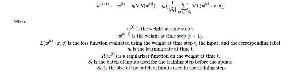
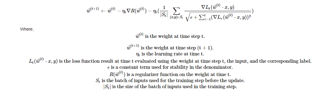
From the equation above, we can see that the intent of the weight updates is to minimize the sum of the loss on the inputs in the training set plus the regularizer function applied on the weights. The purpose of the regularizer function is to penalize the use of large weight values in the model. In the PyTorch library, this shows up as a weight decay parameter in the optimizer. At each time step, we utilize the derivative of both functions with respect to each weight to step in the direction towards which the two values decrease. The step size is determined by ηt , which is controlled as the learning rate parameter. Determining an appropriate value for the learning rate is a balance between the rate of convergence of the model and avoiding over-stepping past the optimal value possible. This specific equation of SGD is applied on some batch of values St at each time step, and the gradient of the loss function is taken as the average of all of these gradients. However, the sum of the gradients for all of the inputs could also be utilized by removing the 1|St| term from the expression.
In training our model, we found this to be helpful in having the model converge to a higher accuracy. The use of batching inputs as opposed to one at a time is a compromise between updating weights based on all data points (gradient descent) and updating the weights based on random samples from the population (which is how SGD normally works). Batching helps maintain the randomization of inputs used for the weight updates from single-input SGD while converging at a similar rate to gradient descent without having to utilize all of the data points for each update step. By repeatedly applying this weight update for different samples from our population of data across several iterations, the model weights are able to approximate the expected labels for inputs.
After taking a look at how SGD works, now it is easier to understand how AdaGrad builds on top of the SGD algorithm. Depending on the representation and range of values of different features, the gradients for each of the features can vary significantly in magnitude when compared between the different features. If non-informative features result in significant gradients along that feature, then this can affect the ability of SGD to converge to an optimal solution. As a result, AdaGrad utilizes the history of observed gradients in the update process to scale future updates of the weights based on previously observed weights. The equation for AdaGrad is presented below:
From the equation, we can see that the AdaGrad algorithm adjusts the influence of features with large gradients by penalizing them with a large denominator term while similarly incresing the magnitude of features with small gradients by having a small denominator term. This algorithm generally helps prevent the weight of the model to travel in the direction of a feature which does not provide any meaningful contribution to the optimal value of the weight and instead towards an optimal solution. As a result, this helps the performance ofthe model to converge faster and reduce the influence of features which do not significantly contribute to the expected output, reducing the risk of overfitting the test data. As a result, we decided to utilize AdaGrad for our optimization algorithm for training the model.
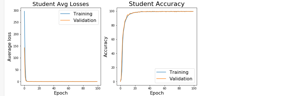
The model_train function was utilized to train the model. Note that the predictions and outputs were multiplied by 100 before being passed into the loss function. Since our predicted values are in the scale of percents represented as decimals rather than whole numbers, we needed to multiply the values by 100 to change the magnitude of the loss to correspond to the numerical percentage value for the gradients to have enough effect on the weight parameters. Since we are solving a regression problem rather than a classification problem, we define correct predictions as being within 0.5% of the expected output by value.
The code following the model_train function is the setup utilized to train the model using PyTorch. This includes defining a dataset to set up randomized data selection, data extraction from the csv files we generated earlier and how the global means and stardard deviations for different parameters were computed. When training the model, we set up K-Fold Cross Validation with SKLearn for each epoch (iteration of training) to separate a random section of the inputs for validation while training on the rest of the data as a training set. We utilized 10 folds to make the train/validation split of the data, separating 10% of the dataset to evaluate the performance of the model each time after training on the remaining 90%. The SKLearn function gives 10 of these splits by setting each one of these folds as the validation split of the data one at a time, and we use all of them, meaning that within each epoch defined in the notebook we run through the data 10 times.
When we ran the code, we obtained the following plots.
After training the model up to a point we are satisfied with its performance, we need to extract the parameters from our model so that we can pass the results to the FPGA. We use the following code block below to write the parameters over to a CSV file based on a format we agreed on for communicating between the HPS and the FPGA once the csv file is parsed.
When we decided on creating a neural net for our project, there was a lot of mystery over how we would implement the neural net on an FPGA. Any idea for the design was further complicated by the fact that we would not know the actual size of the neural net until much later in the design process. Also, the HPS code would be the limiting factor for our speedup in this implementation, so our FPGA design would not need to be highly optimized. Therefore, we decided to take a more conservative approach to implementing the neural net by implementing a reasonably high level of parallelism rather than a pursuing the highest performance design. Taking these measures gave us the confidence that we would get good performance while not running the risk of having the neural net not fit on the FPGA.
Early on, we knew that our neural net would probably have a second layer that was far wider than the other layers, so we decided to parallelize all calculations along this middle layer. We would also need a second module to tie together all the calculations from the parallelized middle layer and present an output. So, our design consisted of two major modules which will be discussed in detail in the next couple sections.
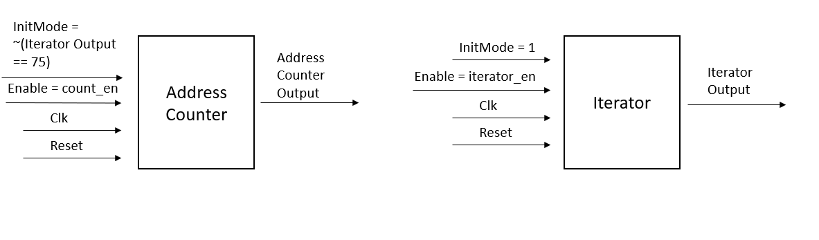
Each node in the second layer, referred to as the Middle Layer, was responsible for multiplying the weights for all the corresponding inputs and summing these values with a bias value. Then this sum needed to be multiplied by all the weights from the Middle Layer node to the third layer node. We decided to corral all this calculation for each Middle Layer node into one module called the neuralnetmiddle. neuralnetmiddle effectively takes in as many inputs as there are nodes in the first layer and outputs as many signals as there are nodes in the third layer. Each neuralnetmiddle module consisted of a fixed-point multiplier that was responsible for computing all the multiplications. We decided to go with a single multiplier for each neuralnetmiddle module because we were unsure of how many nodes would be in the Middle Layer and we did not want to run out of multipliers. The multipliers and the rest of the calculations on the FPGA were conducted with 4.23 fixed point because the DSP blocks that held the multipliers were limited to a resolution of 27 bits. We chose 3 non-decimal bits and 1 signed bit, because some of the weights required 3 bits to represent the non-decimal part of the number. All the calculations happened with the help of a state machine that will be covered shortly.
One of the significant challenges to implementing a neural net in hardware is having a fast solution for storing and reading weights for the neural net. Each neuralnetmiddle module is responsible for storing one 1 bias value, the weights corresponding to the first layer nodes, and the weights from the Middle Layer node to the third layer nodes. To account for all these weights, we implemented a M10K RAM block within each module to store all the nodes. Writing the weights into the RAM block will be discussed in a later section but both writing and reading from the RAM required the use of an address counter. The address counter was implemented in such a way that the counter would overflow after reaching a value that corresponded to the index of the last weight in the M10K block. Writing to the M10K block happens in the first state and the values are read from the M10K block at every subsequent state.
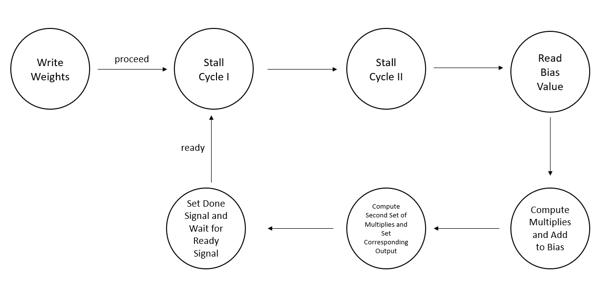
As can be seen in Figure 5, the state machine inside neuralnetmiddle consists of seven separate parts. The Write Weights stage is where the weights are written into the RAM module. Stall Cycle I and Stall Cycle II are used to handle the two-cycle read delay for the M10K RAM. Note that address counter is at zero in Stall Cycle I and is incremented in both Stall Cycle I and Stall Cycle II. So, the data at address 0 can be read the cycle after Stall Cycle II, and every weight can be read in order in all the subsequent cycles as well because address counter is incremented every cycle. Read Bias Value is the stage right after Stall Cycle II and that is where the data at address 0, which holds the bias is read into a register. The Compute Multiples and Add Biases part of the diagram consists of as many cycles as there are inputs to the neural network. In each of these cycles, one of the multiplies corresponding to the input and its weight is computed in a single cycle using the multiplier. The product is also added to the running sum that includes the bias value within the same cycle and stored in the register that initially held the bias value. Once all the sums are computed, the second set of multiplies corresponding to the third layer are computed in multiple cycles, but each multiply is written to an output that corresponds to each node in the third layer. Within the first cycle of these calculations however, the ReLU operation for the Middle Layer is computed. If the sum is less than zero, then the register holding the sum has a zero written to it, which will be used in all subsequent calculations. Once the calculations are complete, a done signal is raised and the neural net waits for the next set of actions.
The neuralnetmiddle module was initially unit tested by using the address counter to write the value of the address at each address in the Write Weights stage. Then the outputs of the neuralnetmiddle module were checked on ModelSim for varying number of first layer and third layer nodes to ensure that the outputs corresponded to the values written into the RAM. Since the numbers we were writing into the RAM were small, simple values, we could quite easily verify the results to ensure that this module was working correctly. Once we reached correctness with this module, we moved on to generating neuralnetmiddle modules to create a larger neural net.
Creating a larger neural net was rather simple conceptually as we would have to generate as many neuralnetmiddle modules as there were nodes in the Middle Layer. Then, we would have to sum up all the outputs corresponding to each node in the third layer from all the neuralnetmiddle modules. Finally, we would have to compute the last set of weight multiplications, sum them up with the bias, and provide the output. However, further questions about the structure of the neural net raised uncertainty about certain parts of the weights. We once again decided to follow out mantra of keeping it simple by just deciding to hardcode the values for the weights and bias into the main module. We figured that the third layer would be rather thin, so it did not make sense to use a RAM to store these weights. We also went with a single 4.23 fixed point multiplier once again because we were unsure of how many multiplies would be taken up by the neuralnetmiddle modules.
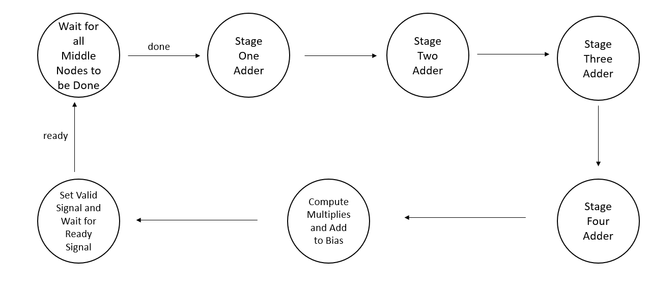
Figure 6 depicts the state machine used to compute the final output. The first stage in the state machine, Wait for all the Middle Nodes to be Done, waits until all the done signals from each of the neuralnetmiddle modules have gone high. A simple bitwise AND allowed us to combine all these signals into one Done signal that could be monitored. The next four stages refer to the four-stage adder that we built to break up the addition of all the previous stage outputs. Because we eventually decided to go with a design that has 75 nodes in the second layer, we would have to compute a 75-value sum for each of the outputs from the second layer. Such a large sum would almost definitely not meet timing and such a large adder might not even be able to be fit onto the FPGA. So, we broke up the sums into smaller chunks of 25, 25, 15, and 10. These values were experimentally derived while trying to make the design fit on the FPGA. On the final stage of the adder, the ReLU operation was computed for each of the sums.
The very last set of computations is quite similar to the first set of multiplies and adds in the neuralnetmiddle module. Each of the sums is multiplied by a corresponding hardcoded weight and added to a hardcoded bias. Once all the sums were computed, the state machine progressed to the last stage where it raises a valid signal for the HPS to see. Testing for the main module was also quite similar to the testing for the neuralnetmiddle module. Simple integers weights were added to the main module and the corresponding output was checked on ModelSim to see that the design does work as intended.
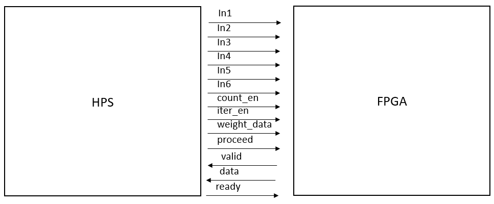
The HPS to FPGA communication was arguably the most complicated aspect of the whole implementation and relied on three different parts: streaming in weights to the neuralnetmiddle modules, reading output from the HPS, and setting up the VGA interface. The inspiration for the first part was derived from Lab 2 where weights for the drum were streamed into the FPGA. To make this implementation work, we had to make some subtle changes to the counter module used by the address counter. Mainly we had to incorporate an InitMode signal, that when high, will make the enable signal for the counter a rising edge enable. The address counter in each neuralnetmiddle module is initially in init mode until all the weights are streamed to the HPS. The counters then progress to normal mode where the counter counts up when the enable signal is simply high. On top of the address counters, an iterator counter is also used to control the whole interaction. As can be seen in Figure 7, the iterator is simply used to iterate through each of the 75 neuralnetmiddle modules. The InitMode setting of the address counter is controlled by the iterator while the iterator is always in InitMode. The enable signals for these counters can be found in Figure 8, which depicts all the signals going between the HPS and the FPGA. The count_en signal is used to provide the rising edge enable to the address counter so that it counts up when a new weight is passed in through the weight_data signal. The iterator_en signal is the rising edge enable signal for the iterator counter and it is used to move on to the next Middle Layer node after all the values for the current Middle Layer node have been streamed in. Since all the address counters in each of the neuralnetmiddle modules would technically count up at the same time, the write enable signal for each of the RAMs was configured to only go high when the iterator counter had reached the value corresponding to that particular node. Finally, the proceed signal from the HPS is used to trigger the neuralnetmiddle modules to move on to Stall Cycle I once all the weights for all the Middle Layer nodes have been streamed in.
One advantage of using this technique to stream values in from the HPS is that the FPGA counters can be controlled from the HPS while the counters still run on the FPGA clock. Using a rising edge enable allowed us to precisely trigger exactly when each operation in the FPGA would happen without having to mix or gate clock signals. So, we relied on the same philosophy to control how the HPS informs the FPGA to compute a new value based on the inputs. The ready signal shown in Figure 8 is used as a rising edge triggered signal. When the FPGA writes output to the data line and raises the valid signal, the HPS can go in and read the data, set new inputs, and raise the ready signal. And when the ready signal is raised, the FPGA triggers all the state machine to go back to their initial state and begin computing on a new value.
Finally, the 16-bit color graphics primitives example project available on the course website was used as the base for all Verilog implementation. This project came with the SDRAM and VGA subsystem setup in the Qsys tool and writing to the VGA display involves first writing to the SDRAM. The VGA subsystem reads data written to the SDRAM and outputs it on the VGA display. The color information of each pixel was represented over two bytes, and each pixel’s data is stored sequentially in the SDRAM. Since the VGA display is a 640x480 resolution display, the location of a specific pixel’s data within the contiguous chunk of memory is determined by the expression: ((640 * y + x) << 1) where y and x represent the pixel coordinates.
The HPS code supported the FPGA by passing in weights and inputs as well as displaying the outputs of the FPGA, graphing the tire degradation on the VGA and displaying the information of each driver in a table on the terminal. The terminal takes in user input for which race it would like to follow, where the user puts a three letter abbreviation for the race they want to select (for example Aus) and then enter a number to pick a driver to follow (ex. 33 for VER). The driver number is used in the code to get the index of the driver and also their initials and displays it on the output. The tires are initially set to 100% since they are fresh tires at the beginning of the race and the arrays containing simulation data for the specific lap and inputs for the neural net are initialized. The user selected race is used to initialize the path needed to pull CSV files for the simulation and inputs. The HPS parses the CSV file (see below) to store into a 2-dimensional array and uses this data structure to send weights to the FPGA, using iterating through the weights as previously described in the FPGA section for passing in weights.
The parseCSV functions are used to extract elements from three different types of CSV files. These are kept as three different functions for simplicity of each individual one, although parseCSV_sim() is very similar to parseCSV_inputs() since both of these only parse a specific row on the CSV. ParseCSV_weights differs from both these functions since weight data is not needed in real time (only for initializing the neural net) and thus it parses through the entire file and stores all this data into a 2-dimensional array. Meanwhile, parseCSV for inputs and simulation data will iterate through the file until it reaches the row specified and then stores the data of only that row into an array, since each row is needed sequentially. When the row specified hasn’t been reached in the file, it signifies that the end of the file has been reached and thus the end of the race, signaling done_race high. Aside from this, parseCSV functions very similarly. It takes a data structure as an input to store the data parsed and also the path of the file to parse. It opens the file (returning an error if unsuccessful) and stores each line into a temporary char array that is split into different entries based on the delimiter “,” (because of the properties of CSVs, comma separated values) by using the function in the string.h library “strtok”. The entries are converted to a float using the “strof” function and stored into the data structure. The next entry is found by calling strtok again until it outputs NULL, signifying the end of the line as no more entries are found. When this happens, the function parses the next line and the process of separating the parsed line into entries restarts. Once complete, the file is closed.
A flag called done_race was used to signify if the race was finished to end the program. A loop was created for when done_race is still 0 (not finished) to start and continue the simulation of the race. The program then parses the subsequent row for inputs of the neural net and simulation data and the inputs are passed into the FPGA using a valid ready protocol as previously described in the FPGA section for taking in inputs. The driver number derived from the row of simulation data was used to index the current driver to be able to update accordingly with the new data of the specific lap. The simulation data will set a weather flag from the simulation data to be set to 1 if not raining and 0 otherwise, to be displayed as context to the user. Additionally the simulation data indicates if a pit stop was taken or if a driver did not finish, and the flags internally are modified accordingly. For example, if the selected driver by the user took a pit stop, a flag is raised so the user can be notified of the pit stop on the next lap. All drivers that take a pit stop have their tire degradation reset to 100% since they are now operating on new tires. Once a new lap has been taken (the current lap is greater than the previous lap) the data is updated to the user on the terminal with the new lap number and previous tire degradation of the driver being followed. Information about each driver is printed as each row of simulation is parsed— along with the new tire degradation data derived by the FPGA output— until this new lap flag signals to delay for three seconds before printing a new table with new headings. This delay is solely used to ensure the user can read the results of the current lap before the information is updated. More information on what is printed can be found in the results section. If the simulation data is currently about the driver selected by the user, the new tire degradation point will be graphed on the VGA.
To get the tire degradation of each driver, getTireDegr(), the output of the FPGA (again extracted based on the valid ready protocol) is converted to a float and multiplied by 100 to get a percentage. In order to increase the resolution for graphing, this number is multiplied by two to get 0.5% resolution. It is cast into an integer and negative numbers are set to zero. This result is the change in tire degradation in that current lap. To get the overall tire degradation, this result is subtracted from the previous tire degradation.
The fix to float conversion works similarly as float to fix by dividing by 2n ,where n is the number of bits to shift right. Since we are using 4.23 notation in our fixed point numbers, n is 23. One edge case that we had to adjust for in this was how right shifting loses the MSB, so we had a conditional check that would subtract 16 from the value of the quotient was greater than 8, essentially subtracting this MSB to make it negative.
To graph the tire degradation, first a horizontal line was drawn near the bottom third of the screen to signify 0% tire degradation (where we recommend changing tires) by using the VGA_PIXEL macro to graph each pixel from x = 40 to x = 599. This was done before the start of the race simulation. The graph plots the new tire degradation for the selected driver. It gets the tire degradation value for this driver by calling the function getTireDegr(), mentioned above and then VGA_draw_helper() is called to actually plot on the VGA. This function will map the new point to be plotted into pixels for the VGA. In order for there to be a noticeable difference for the user to see, each increment in the x value (number of laps) is mapped by 6 pixels. This increment is added to an x offset to ensure it isn’t on the edge of the screen. Given that the total possible laps is 100, this would make the maximum x be plotted to the 600th pixel horizontally, extending the range of the graph. The vertical pixels are derived from the tire degradation value stored subtracted from a y offset corresponding to the location of the horizontal line drawn. Since 0 is the top pixel of the screen, this ensures that increasing tire degradation means the graph plots upwards and decreasing degradation plots on lower parts of the graph. To draw clear distinct lines when a new tire degradation has been output for the selected driver, VGA_line is called to plot a line between the previous tire degradation and the current degradation. The current pixels found, x and y, are then stored as prev_x and prev_y after this function call. During the first function call when no degradation values have been plotted yet, prev_x and prev_y are x_offset and y_offset respectively. A stop flag is used if the count exceeds 100 to ensure it doesn’t plot beyond the 600th pixel. Since there can’t be more than 100 laps, this won’t be reached but is kept as a redundant check. An array was used to store the data being plotted with the intention of storing the plots of other drivers in similar data structures, so that the user could specify in the middle of the program to change to the plot of another driver. This functionality has not been implemented, but is another step that could be added to extend functionality in the future.
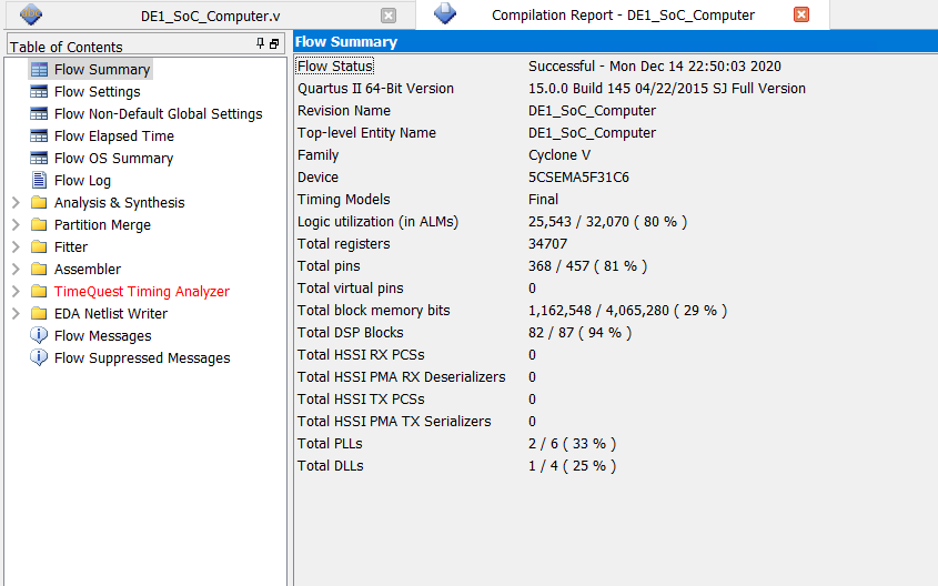
Figure 9 shows the Compilation Report for the final design implemented on the FPGA. The most apparent thing from the report is that the number ALM usage is almost at eighty percent, which was an initially surprising result for us. Lab 2, which consisted of a large design, used approximately the same amount of ALMs, so we were a little unsure about where the bottleneck seemed to be coming from. But after placing some thought into the issue, we came to the realization that although our Lab 2 design was larger, it used relatively few adders for such a large design. For this project however, there was a significant amount of adder resources required at almost every stage of each stage machine. While we envisioned all the additions within the same module happening on the same adder, it is quite possible that each stage used its own adder. In retrospect, it is quite fortunate that we decided to go for a more conservative approach when implementing the neural net on the FPGA. If we had relied on a more aggressive design, it is likely that we could have overextended the number of ALMs available on the Cyclone V SOC. Nevertheless, the design was able to properly read in the various weights and provide the necessary computations for the neural net. The output of the FPGA neural network matched the Python program to six decimal places, so we were able to reach a high level of precision with this system. Also, the design computed values at a deterministic thirty-seven clock cycles, which on a 50 MHz system is certainly in the realm of real time computation. We did not take any measurements of the runtime on the FPGA because the HPS interactions themselves would have contributed to most of the noise in the system, which in and of itself is a testament to the speed of the design.
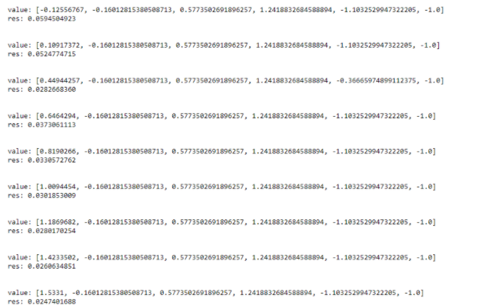
To test the functionality of the complete design, we ran both the FPGA model and the Python model with the same inputs and utilizing the same weights. When we created the Python model in PyTorch, we saved the model to be able to reload it at a later time to extract the parameters again if necessary. This was also useful for testing since we can load the trained weights onto a PyTorch net and be able to run through inputs to observe the expected outputs. In the main jupyter notebook file where we developed the model Final Project, we include the necessary code to save the model, reload the model, and to evaluate a sequence of inputs and print the observed outputs.
Since we intentionally designed the FPGA model and the Python model to have the same design and weights, we expected to observe the same results. In developing our design, we initially found that these values did not correctly match each other, so we knew that a bug existed in our design. After going through the implementation, we found that an additional assignment to the cumulative sum at the middle node was present. This resulted in the ReLU activation function present in the Python model to not be executed correctly for the FPGA model. After making this correction, for the data points we ran for our races we found that the two models returned very similar results, with up to 6 decimal points of precision when comparing the two returned values. To run the race data points in a way that we could easily compare our results in the FPGA and the Python models, we utilized a separate HPS test code TestWeights.c which prints out the input and the corresponding output values. In the jupyter notebook previously mentioned it can be seen that a similar format was utilized. However, if the cells are run sequentially then the results for all of the races will be displayed in the notebook while the C code runs only for data from a specific race.
While we developed the design for the neural network model with processing speed of the inputs in mind, we decided to not explicitly calculate the necessary amount of time required to process inputs. Since our project was designed around returning results on a lap-by-lap basis rather than real-time, we do not need the design to be able to compute these results at a significant speed. Rather, we have to throttle the speed of the FPGA model by delaying when we feed inputs into the neural network such that the results of the simulation are viewable at an appropriate rate. As long as the results are returned to us in a timely manner, for the purposes of this project this was sufficient. We did not chase for perfectly optimal execution of inputs, but rather a sufficiently parallel and functional design for implementing the neural network on the FPGA. Since the speed of execution of the model was not our focus but rather the ability to embed such a device within an FPGA, and the design of our model in how it operates does not depend on the speed of execution, we exclude measuring the processing time of inputs before we receive back an output.
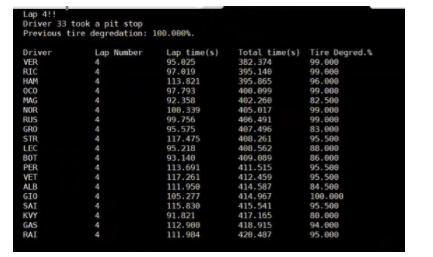
Our system displays the results on two locations. The terminal and the VGA. As a result of the simulation being run, every lap is displayed with information about the current lap number, if it is raining or not, and for the driver being followed: their previous tire degradation, if they took a pit stop, and if they didn’t finish the race. An example of a lap with a driver taking a pit stop is shown below.
When the selected driver does not finish, a DNF flag is set to display the user that the driver is out of the race. All other drivers that have not finished have their times set to -1.
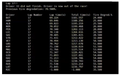
As seen in the image, the scoreboard displays the driver initials, the lap number, the lap time, total time, and the current tire degradation. In addition to this terminal output that updates every lap, our monitor is updated from graphing on the VGA the tire degradation of the driver selected as seen here. Note that whenever a pit stop is taken, tire degradation immediately jumps to 100% as the driver now has fresh new tires. The tire degradation was verified with the expected tire degradation of the python model and was found to be a match for the columns we selected for different tires in different laps, demonstrating correct functionality.
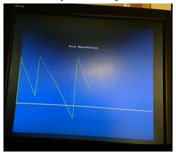
Another important note is that the plot shows tire degradation being negative here. This can be attributed to the fact that our tire degradation estimations predict when tires should be changed and 0% corresponds to when pit stops are expected to be taken, not when tires are fully worn. This discrepancy means that sometimes drivers may continue extra laps even on subpar tires based on differences in strategy from our model.
Our design is capable of being used by other users for either the same dataset or other datasets from races that we did not decide to cover, with some limitations to precision and freedom of adjustability. For the data collection process, we included our process for what data needs to be defined and how it is separated into both simulation data and input data for the neural network to create additional datasets, whether based on real races or simulating fake races. Similarly, we provide our structure that we defined to train our neural network model that was later implemented in the FPGA. However, there are two main limitations in the flexibility of our design in how this was currently implemented. First, the layout of the neural network is fixed in the FPGA design, therefore the activation functions and number of nodes or layers cannot be adjusted without also adjusting the FPGA implementation. Second, the weights from the second hidden layer to the output were hard-coded for practical purposes, as we intended the design to be static once implemented. While a new model could be trained on a different set of races and new weights can be obtained, the hard-coded weights in the FPGA implementation would have to be adjusted accordingly. However, the remaining weights are simply read off a csv file, thus they do not require any additional modification beyond generating the csv file with code we include here. Beyond these limitations, other users are also able to utilize our model.
At the conclusion of this project, we fully completed the different components of the project and we were able to predict our labeling equation for tire degradation much better than we originally expected. Both the ability of the neural network model in Python to be able to reach such a high accuracy in prediction level for a regression model and the FPGA predictions being essentially equal to those from the Python model exceeded our expectations from when we first planned on executing this project. We were concerned that there could be potential issues when transferring our model to the FPGA such as loss of precision in values for intermediary calculations and the risk of overflow at any point in the computation, which would significantly alter the prediction results. While both issues may still be present, we did not observe these when running through our datasets.
In the future, we could further improve on this project by progressing towards the use of real-time data coming directly from the car, as we originally imagined for this project before compromising with the simplifications made. This would involve ensuring the speed of the predictions is sufficient relative to the rate at which data is received from the car sensors while maintaining some high level of accuracy. At the same time, such a neural network layout would likely require more complex layer operations instead of a simple feed-forward neural network, such as a recurrent neural network. This would require maintaining a short memory within the FPGA for each node of the previously observed values at the node to determine the output at the node along with the input values at that time.
Another future issue to be addressed from this project is the issue of determining the observed tire degradation, whether it be on a lap-by-lap basis as this project or in real-time for the model suggested above. Due to the constraints of time and data availability for this project, we made significant simplifications to this process to emphasize the neural network implementation on the FPGA. However, if we want a more precise model of the tire condition of drivers, then the simplifications we made for this project have to be accounted for and possibly a more precise mathematical model for tire degradation could be developed. Some of these factors to take into account include finer lap time breakdown, weight loss due to fuel consumption throughout the race, effects on tire condition of locking up the tires under braking or blistering of the tires from overheating, and individual tire conditions for each tire in the car.
With respect to the FPGA itself, we believe that a larger FPGA could have potentially alleviated some of the design concerns that we were facing. Having many more ALMs would have allowed us to be more aggressive with our parallelization while not worrying about the design fitting on the FPGA. Also, having many more multipliers would have let us reduce the serial portions of our state machine significantly. This leads us to conclude that an FPGA on its own might not be the most apt hardware structure for building a neural network. Rather, a programmable hardware system with a large array of multipliers and adders would have been optimal for this project. While ASICs that are capable of such a design exist, they are often hardwired not as extensible as an FPGA. Instead, we need a hybrid design between ASICs and FPGAs to allow us to eek out maximum performance from this system.

Felipe Shiwa
Felipe worked on designing and training the neural network. This was done in Python utilizing the PyTorch library to create and train the model. He also collected the data utilized for the project and parsed the data into the inputs for the simulator and the neural network.

Sujith Naapa Ramesh
Sujith wrote all the Verilog for the project; he implemented the neural network on the FPGA and also built the FPGA to HPS interface. Sujith also designed this website.

Rishi Singhal
Rishi worked on the HPS code for the project. He wrote code to parse the CSV files and send the neural net information to the FPGA and take the output to plot tire degredation on the VGA monitor and display tire degradation and the current standings of each lap on the terminal
Neural Network node image adapted from CS 4780: Introduction to Machine Learning lecture slides.
ReLU Graph Created on Desmos.com
Pytorch Documentation and Tutorials
Base code from CS 4670: Computer Vision Spring 2020 Assignment 3
Learning Material for CS 4780: Introduction to Machine Learning
The group approves this report for inclusion on the course website. The group approves the video for inclusion on the course youtube channel.
Python Code
Verilog Code
HPS Code