Julia Set Renderer
Table of Contents
Introduction
The Julia Set Renderer is a combination of compiler and a custom VLIW processor/supporting framework running on an FPGA. Julia sets are fractal shapes which are generated by iterating a point's coordinate according to an update rule (a function which must be a rational polynomial) for every point in the complex plane. Under that iteration, the value will either diverge to infinity eventually in which case it is not considered in the set, or have a magnitude bounded by a some constant in which case it is considered in the set. The Julia Set Renderer makes that determination for each pixel in a 640x480 VGA display by mapping each pixel to a point in the complex plane and iterating each point according to a user-supplied formula.
This project gives the user an interface via an ssh terminal in which to type a formula (for example \(z^2+c\)) and draws the corresponding Julia set on a VGA screen. The user can use a mouse to pan/zoom around the drawn set.
Architecture
I started with my implementation of a solver for Lab 4 - Mandelbrot Set. My implementation used 27-bit, floating point arithmetic to draw regions of the Mandelbrot set by mapping each pixel to a coordinate in the complex plane and determining whether the iterated equation \(Z_{n+1} = Z_n^2 + C\), where \(Z_0=0 + 0i\) and \(C\) is the coordinate corresponding to the pixel in question, diverges. The color of the pixel is determined by how many iterations it took for \(Z\) to have magnitude greater than a threshold, capped at 1000 iterations.
For that project, implemented on the DE1-SoC development board, I used the HPS (an ARM processor connected to the FPGA fabric via an AXI bus) to handle the UI components including the mouse updates, and the FPGA to fill the VGA framebuffer with colors based on how long it took the point to escape. The HPS updates the parameters in the FPGA used to map the pixels on the screen to complex coordinates based on the user inptus to enable the interactivity.
In the Mandelbrot set project, my solver iterating the equation for \(Z\) was static and hand optimized for the given equation. In this project I replaced that solver with a VLIW CPU designed to support a limited set of floating point operations that could be used to iterate arbitrary equations (see VLIW Processor). I also wrote a compiler which produces instructions to be run on the VLIW processor given the equation of a Julia Set (see Compiler).
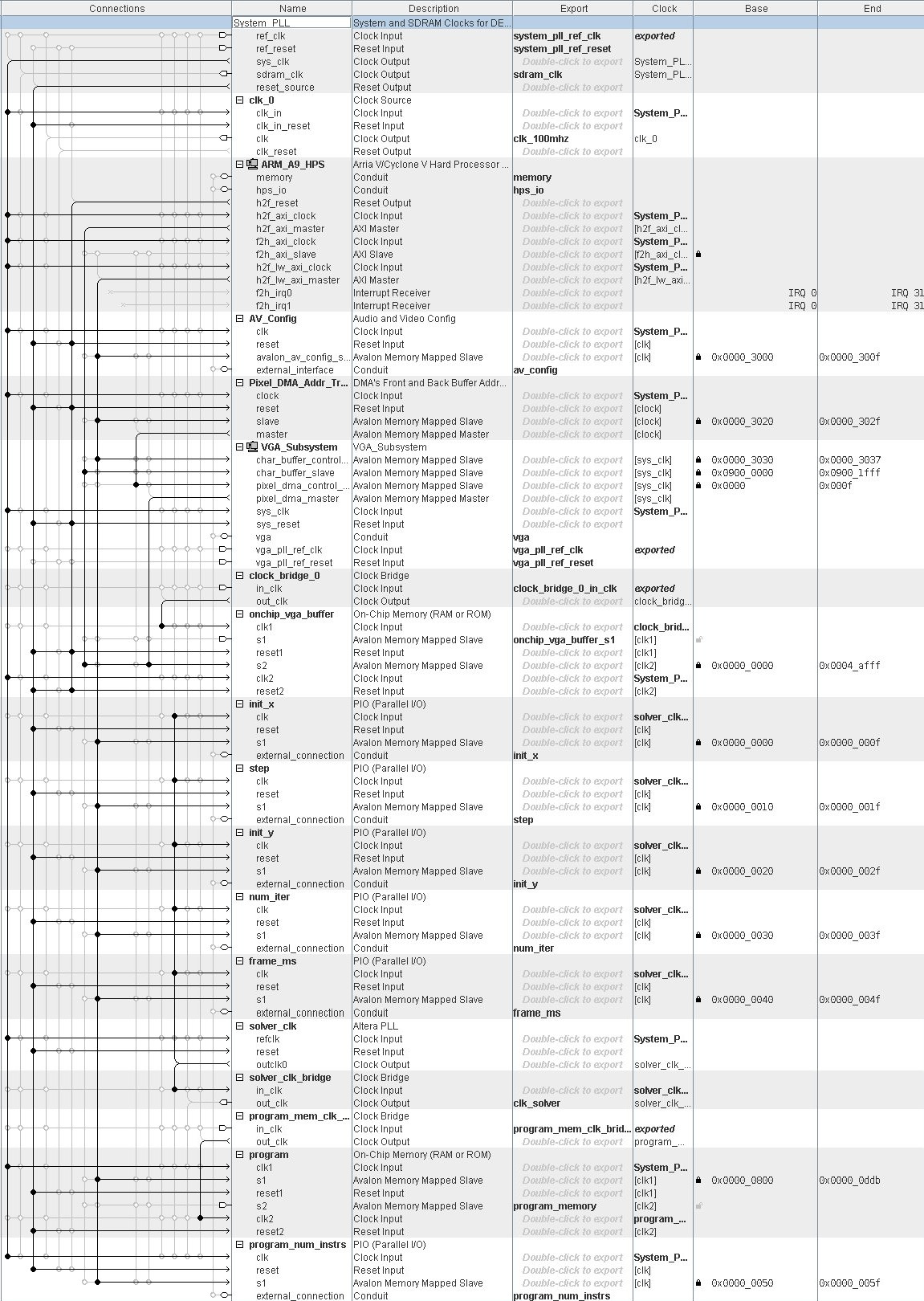
Figure 1: Project Architecture
I will first describe the architecture of the FPGA-side framework that sets up the VLIW processor to solve a particular pixel, then the HPS-side UI components, and finally the heart of this project - the VLIW processor and its compiler.
Framework (FPGA)
Pixel Solver
The pixel solver, a shim around the the VLIW processor, provides an interface
for controlling the VLIW processor. Interfacing with the pixel solver entails
setting the instruction on each cycle and waiting for the done interrupt to be
thrown. On the same cycle that the inputs are ready a start signal is strobed
which sets off the computation. When the solver is done (the magnitude of \(Z\)
has escaped), it strobes the outut done (effectively sending an interrupt).
Row Solver
The row solver instantiates a single pixel solver, but provides an additional
abstraction. The row solver accepts C_B which is the imaginary component of
the row to be operated on. Additionally, it accepts C_A_reference which is the
real coordinate of the leftmost pixel in the frame (floating point), C_A_step
which is the step size between pixels (floating point), and generates the index
C_A_column (10-bit unsigned number). Together, those specify the real
component of the point's location by the expression \(C\_A\_reference +
C\_A\_step * C\_A\_column\). The row solver uses the VLIW CPU to evaluate that
expression to determine the pixel's coordinates, then iterates the given program
on that pixel coordinate until the magnitude diverges or the maximum number of
iterations is reached.
The Row Solver uses the VLIW CPU to calculate the pixel's coordinate is an optimization which allows using the solver's instantiated adder/multiplier instead of instantiating new ones as resources on the board are in high demand.
The row solver supplies the pixel solver with the necessary inputs, starting at
column 0. When the pixel solver throws an exception indicating the magnitude of
the iterated equation has escaped the threshold or when the Row Solver
determines that the maximum number of iterations has been reached the iteration
count and location of the pixel is strobed out from the Row Solver. If the end
of the row has not been reached, the Row Solver resets the Pixel Solver and
repeats the process for the next pixel. Otherwise, if the end of the row has
been reached, then the Row Solver sets its request signal and waits for the
grant input to be strobed indicating it should start on the next line.
Frame Solver
The frame solver accepts the coordinates of the top left corner of the screen
and the step sizes for the real and imaginary axes. The frame solver
instantiates row solvers and coordinates the inputs and outputs to/from each. At
most one row solver is given a grant in a particular cycle (so it takes at
least as cycles to get the row solvers all computing as there are row
solvers). On any cycle when at least one row solver's request flag is set high
the lowest indexed row solver whose request is high receives a grant and
gets assigned an imaginary coordinate corresponding to the row it should start
computing. The imaginary coordinate is incremented by the imaginary step size
using an adder. If no row solvers are have their request flag set then no
action is taken. If the row index exceeds the frame size then it is reset to 0
and the running count of the imaginary coordinate is reset to the initial value
(that of the top left corner).
The output of each row solver is fed into a corresponding true dual-ported FIFO. Each time the row solver strobes its output signal the coordinates of the most recently generated pixel and the pixel's value are concatenated and inserted into a FIFO.
On a separate clock domain, the outputs of the FIFOs are arbitrated and used as
the outputs of the frame solver. On each clock cycle on the output_clk
domain a pixel's coordinates and value may be output; if one is available on
that cycle then a strobe signal is set high. FIFOs are emptied with those having
lowest index having highest priority. While that is not fair, it doesn't impact
the draw time of the solver since the high-indexed solvers will simply be
blocked when framebuffer bandwidth is the limiting factor and since solvers are
not pre-assigned rows a subsequent change in the cause of the bottleneck would
not disproportionately leave some solvers "out of work".
Top Level
The top level module instantiates a single frame solver and interfaces it with the HPS PIO signals and the VGA framebuffer. The VGA framebuffer is a dual-ported SRAM with one port dedicated to the VGA subsystem and the second exported from QSYS into Verilog. The output interface of the Frame Solver conveniently wires combinationally into the input interface of the SRAM; each time the frame solver's strobe indicating an output is available is wired to the SRAM's write enable and the frame solver's pixel coordinates combinationally determine the address to which the frame solver's iteration count output should be written. This is by design to minimize logic which can't be unit tested in ModelSim (the top level module is the only module not tested in ModelSim, as is discussed later). The SRAM's value is an 8-bit color which is determined by the bottom eight bits of the number of iterations that point took to escape.
The top level module also keeps track of the number of cycles it takes to compute each frame which is passed to the HPS to display in milliseconds on the display.
The top level module also contains the instruction broadcast code which reads the VLIW instructions from SRAM on each cycle and broadcasts it to each of the VLIW processors. This is repeated "blindly" and the processors subscribe/unsubscribe as needed.
QSys
QSys was used to connect the HPS and FPGA to registers, clocks, RAMs, etc in a graphical layout. The screenshot below shows the layout used for this project.
Figure 2: QSys Diagram
User Control (HPS)
The HPS, running Linux, is responsible for updating the PIO registers with the current frame's top-left-corner position and step size. The user's mouse movements are scaled based on the current zoom and used to update the position, while the left/right mouse buttons increased and decreased the zoom by updating the step size and the top-left-corner position accordingly to keep the image centered during a zoom (otherwise you would be zooming into the top left corner).
The HPS loads the a program generated by the compiler into the program memory when the HPS program is launched. The VLIW program is stored in an array which is simply written to a RAM block.
The HPS also displays the current coordinates and the frame generation time on the display in the text buffer.
Program/hardware design
Compiler
The compiler, written in Haskell, takes an equation for a Julia Set with the variable \(z\) representing \(Z_{n-1}\) and produces an array representing the instructions to be run on the VLIW CPU. When the user launches the compiler they are prompted for an equation, for example \(z*z+1i2\), which represents \(Z_n = Z_{n-1}^2 + 1 + 2i\). They are then given an array which can be plugged into the C program for the HPS which flashes the code to the VLIW CPU's program memory.
The following sections use the above equation as an example in describing how the compiler parses, translates, and assembles programs.
Parser
I used Haskell's recursive descent parser library Parsec to parse the
equations (which lend themselves to recursive descent parsing). The parser reads
the equation into the following algebraic data type:
data Exp = Num Int     -- base numeric data
         | Cpx Exp Exp -- complex numbers, real & imaginary components must be Num
         | Var String  -- only 'z' is permitted
         | Add Exp Exp
         | Sub Exp Exp
         | Mul Exp Exp
         | Div Exp Exp
         | Pow Exp Exp
         | Pos Exp
         | Neg Exp
           deriving (Show)
In the example formula above, \(z*z+1i2\), the parser returns this result:
Add (Mul (Var "z") (Var "z")) (Cpx (Num 1) (Num 2))
IR
The parsed expression is then converted into an Intermediate Representation
where each node in Exp is translated into one or more Instruction objects.
data Instruction =
  --     SRC1     SRC2     DEST
    Add  Register Register Register
  | Mul  Register Register Register
  --     SRC      DEST
  | Neg  Register Register
  --     Val      DEST
  | Load Int      Register
  --     DEST
  | Var  Register
                 deriving (Show)
The translation to instructions has the below signature, where the output is a
Complex (defined type Complex = (Register, Register)) indicating where the
result of the computation will be stored, and a list of instructions. The
instruction output is a nested list where the first sub-list represents the
LATEST instructions to be run. If two instructions could be run concurrently
(dependency wise, not hardware wise) then they may exist in the same
sub-list. The result is how the program could be executed in the fewest possible
number of cycles assuming there were infinite copies of each pipe available in
the CPU.
preschedule :: JuliaParser.Exp -> State Int ([[Instruction]], Complex)
The next step is to convert the instructions to cycles, which have a notion of
the hardware constraints. There are four fields in Cycle which correspond to
the four pipes in the CPU. If a pipe should be starting an instruction in a
particular cycle then that instruction should appear in the appropriate
field. If no instructions start in a pipe in a cycle then the field is set to
Nothing (see Haskell's Maybe monad for a description of how that works). The
flattenSchedule function takes the nested-list-of-instructions data and
schedules it into a list of Cycles. The key to flattening the 2d instructions
into the 1d schedule is the intuition that every instruction appears at the
lowest index possible (i.e. running as late as possible chronologically) in the
input, but it could certainly be executed earlier as long as all of its inputs
are ready (I assume a large register space so there are no collisions). A
trivial way to ensure there are no Read After Write dependency violations from
scheduling instructions earlier I guarantee all instructions that came earlier
than instruction \(I\) in the 2d instruction list have already run by the time \(I\)
is executed.
data Cycle = Cycle { load :: Maybe Instruction
                   , add  :: Maybe Instruction
                   , mul  :: Maybe Instruction
                   , neg  :: Maybe Instruction
                   } deriving (Show)

flattenSchedule :: [[Instruction]] -> [Cycle]
[
  Cycle {load = Nothing,          add = Nothing,                mul = Nothing,            neg = Nothing},
  Cycle {load = Nothing,          add = Nothing,                mul = Nothing,            neg = Nothing},
  Cycle {load = Nothing,          add = Just (Add 4 5 2),       mul = Nothing,            neg = Nothing},
  Cycle {load = Nothing,          add = Nothing,                mul = Just (Mul 0 0 4),   neg = Nothing},
  Cycle {load = Nothing,          add = Nothing,                mul = Just (Mul 1 1 5),   neg = Nothing},
  Cycle {load = Nothing,          add = Nothing,                mul = Nothing,            neg = Nothing},
  Cycle {load = Nothing,          add = Just (Add 4 522 0),     mul = Nothing,            neg = Nothing},
  Cycle {load = Nothing,          add = Just (Add 4 523 1),     mul = Nothing,            neg = Nothing},
  Cycle {load = Just (Load 0 4),  add = Nothing,                mul = Nothing,            neg = Nothing},
  Cycle {load = Nothing,          add = Nothing,                mul = Nothing,            neg = Nothing},
  Cycle {load = Nothing,          add = Just (Add 525 20 523),  mul = Nothing,            neg = Nothing},
  Cycle {load = Nothing,          add = Just (Add 524 19 522),  mul = Nothing,            neg = Nothing},
  Cycle {load = Just (Load 2 20), add = Nothing,                mul = Nothing,            neg = Nothing},
  Cycle {load = Just (Load 1 19), add = Nothing,                mul = Nothing,            neg = Nothing},
  Cycle {load = Nothing,          add = Just (Add 785 784 525), mul = Nothing,            neg = Nothing},
  Cycle {load = Nothing,          add = Nothing,                mul = Just (Mul 1 0 785), neg = Nothing},
  Cycle {load = Nothing,          add = Nothing,                mul = Just (Mul 0 1 784), neg = Nothing},
  Cycle {load = Nothing,          add = Just (Add 274 782 524), mul = Nothing,            neg = Nothing},
  Cycle {load = Nothing,          add = Nothing,                mul = Nothing,            neg = Just (Neg 783 274)},
  Cycle {load = Nothing,          add = Nothing,                mul = Just (Mul 1 1 783), neg = Nothing},
  Cycle {load = Nothing,          add = Nothing,                mul = Just (Mul 0 0 782), neg = Nothing}
]
Assembler
The last step of compilation is converting each Cycle to its 121-bit VLIW
instruction. Each pipe's instruction is encoded separately in a cycle (see the
type signature of encodeLoad below for an example the associated type
signature where BV is a BitVector). If an instruction is Nothing in a
cycle then the code for a NOP is emitted. An instruction word is created by
concatenating the bits together from the individual pipes. The assemble
function maps each cycle to the concatenated instructions of the pipes. The last
step of the assembler is reversing the list of instructions since until now the
lowest-indexed instruction ran last.
encodeLoad :: Maybe IR.Instruction -> BV.BV
assemble :: [IR.Cycle] -> [Word128]
Here is a decimal representation of the list of cycles from our running example:
[
  1073742606,
  1074792207,
  8534579836514498005434368,
  2924556919630725120,
  1073743632,
  1074791185,
  4075231024617881600,
  1329228005872192911768272894028677120,
  1329228015785384632608232126619320320,
  3485829014013083648,
  3488083014997508096,
  0,
  1329227995823601499131475193870942208,
  2316000299778572288,
  2315998098607833088,
  0,
  1074791429,
  1073741828,
  2314861207879680000,
  0,
  0
]
VLIW Processor
The VLIW processor, as was indicated in Compiler, has Load, Neg, Add, and Mul pipes. It additionally has a register file and all the logic required to marshal data to and from registers/pipes as needed.
The processor has a 121-bit instruction format, specified as follows:
load_enable_input- Bit(s) [120]
load_value- Bit(s) [119:93]
load_dest_addr- Bit(s) [92:83]
neg_enable_input- Bit(s) [82]
neg_src_addr- Bit(s) [81:72]
neg_dest_addr- Bit(s) [71:62]
add_enable_input- Bit(s) [61]
add_src1_addr- Bit(s) [60:51]
add_src2_addr- Bit(s) [50:41]
add_dest_addr- Bit(s) [40:31]
mul_enable_input- Bit(s) [30]
mul_src1_addr- Bit(s) [29:20]
mul_src2_addr- Bit(s) [19:10]
mul_dest_addr- Bit(s) [9:0]
Each of the compute pipes can be enabled separately, and when enabled operate on
the given registers with the exception of load which stores a 27-bit floating
point value in the specified register. The neg, add and mul pipes are
implemented with modules from the Floating point hardware on the 5760 page.
The processor has a floating point register file where the first three registers
(indexes 0-2) are special-purpose and the remainder are general
purpose. Registers 0 and 1 are designated to hold the real and imaginary
components of \(Z\) respectively. Thus, the compiled program can count on the
result of the previous iteration being there and is responsible for storing the
result of its computation there as well. In the next section I describe how
\(Z_0\) is loaded into those registers. Register 2 is special-purposed to throw an
interrupt when a value larger than max_magnitude is written to it. The last
thing the compiled programs do is calculate the squared magnitude of \(Z_n\) and
write it to register 2; if the magnitude has escaped the threshold then the
processor sets its done flag high (the VLIW processor takes no further action,
but the Row Solver's response is described next). If two pipes try to write to
the same register on the same cycle the behavior is undefined.
In the current implementation the VLIW processor, each instruction is run for several cycles on each instruction so that the output is set correctly as the add pipe is not combinational. A simple update would solve that, it would just require the add pipe's control signals to be pipelined, and would result in a substantial performance increase.
Row Solver
The Row Solver has four states: a reset/init state, a prelude state, an
instruction_broadcast_sync state, and a compute state. During init the Row
Solver sets ready and waits to be assigned a row to solve. Once received, it
needs to load the imaginary coordinate into the VLIW processor and calculate the
real coordinate on the VLIW processor. To do so it initially runs a hand-written
5-instruction sequence on the VLIW processor:
reg [120:0]                 load_instructions [0:4];
always @(*) begin
   load_instructions[0] <= { // load column_idx --> reg3
                            // ld_en,  val,        dest,
                            1'd1,      col_idx_fp, 10'd3,
                            // neg_en, src,    dest,
                            1'd0,      10'd0,  10'd0,
                            // add_en, src1,   src2,   dest,
                            1'd0,      10'd0,  10'd0,  10'd0,
                            // mul_en, src1,   src2,   dest
                            1'd0,      10'd0,  10'd0,  10'd0
                            };
   load_instructions[1] <= { // load step --> reg4
                            // ld_en,  val,             dest,
                            1'd1,      solver_C_A_step, 10'd4,
                            // neg_en, src,    dest,
                            1'd0,      10'd0,  10'd0,
                            // add_en, src1,   src2,   dest,
                            1'd0,      10'd0,  10'd0,  10'd0,
                            // mul_en, src1,   src2,   dest
                            1'd0,      10'd0,  10'd0,  10'd0
                            };
   load_instructions[2] <= { // load reference --> reg5, mult step*col_idx->7
                            // ld_en,  val,                  dest,
                            1'd1,      solver_C_A_reference, 10'd5,
                            // neg_en, src,    dest,
                            1'd0,      10'd0,  10'd0,
                            // add_en, src1,   src2,   dest,
                            1'd0,      10'd0,  10'd0,  10'd0,
                            // mul_en, src1,   src2,   dest
                            1'd1,      10'd3,  10'd4,  10'd7
                            };
   load_instructions[3] <= { // put B into reg1
                            // ld_en,  val,        dest,
                            1'd1,      solver_C_B, 10'd1,
                            // neg_en, src,    dest,
                            1'd0,      10'd0,  10'd0,
                            // add_en, src1,   src2,   dest,
                            1'd0,      10'd0,  10'd0,  10'd0,
                            // mul_en, src1,   src2,   dest
                            1'd0,      10'd0,  10'd0,  10'd0
                            };
   load_instructions[4] <= { // add reference + offset -> reg0
                            // ld_en,  val,    dest,
                            1'd0,      27'd0,  10'd0,
                            // neg_en, src,    dest,
                            1'd0,      10'd0,  10'd0,
                            // add_en, src1,   src2,   dest,
                            1'd1,      10'd5,  10'd7,  10'd0,
                            // mul_en, src1,   src2,   dest
                            1'd0,      10'd0,  10'd0,  10'd0
                            };
end
Once the coordinates of \(Z\) have been saved to registers 0 and 1 the Row Solver
waits until the instruction sequence being broadcast returns to index 0 (during
which time the processor is executing NOP instructions), and then enters the
compute state in which it forwards the instruction broadcast to the processor
and awaits the processor's done flag. The Row Solver counts how many times the
processor has executed the broadcast instruction sequence which is both used as
the output value (how many iterations it took for the value of \(Z\) to escape)
and is used to abort the computation if it reaches some threshold (nominally
1000 iterations). Once the processor's done flag is set or the maximum number
of iterations is reached, the processor is unsubscribed, reset, and the number
of iterations is stored in the Row Solver's output FIFO.
parameter state_reset=0, state_load=1, state_wait_for_start=7, state_compute=8;
always @(posedge solver_clk) begin
   output_stb <= 0;
   solver_reset <= 0;

   if(reset || state == state_reset) begin
      state <= state_reset;
      start_request <= 1;
      vliw_instruction <= instruction_nop;
      output_value <= 0;
      solver_reset <= 1;

      if (start_grant) begin
         state <= state_load0;
         start_request <= 0;

         output_row_idx <= row_y_idx;

         // start the simulation of the first element of the row
         solver_C_A_reference <= row_x_reference;
         solver_C_A_step      <= row_x_step;
         column_idx           <= 0;
         solver_C_B           <= row_y;
         solver_start         <= 1;
      end
   end
   // load the coords into the regs
   else if (state == state_load0) begin
     // EACH OF THE 5 INSTRUCTIONS IN THE LOAD SEQUENCE ABOVE
     // IS SET HERE FOR ONE CYCLE
   end
   else if (state == state_wait_for_start) begin
      vliw_instruction <= instruction_nop;
      if (instruction_number == 0) begin
         state <= state_compute;
         output_value <= 0;
      end
   end
   else if (state == state_compute) begin
      vliw_instruction <= instruction_end; //vliw_instruction_broadcast;
      if (instruction_number == 0) output_value <= output_value + 1;
      if (solver_done || output_value > max_iterations) begin
         output_stb <= 1;
         // receive results

         // start on new results
         if (column_idx == 639) begin // just finished last column
            state <= state_reset;
         end
         else begin
            state <= state_load0;

            column_idx <= column_idx + 1;
            solver_start <= 1;
         end
      end
   end
end
Frame Solver
The frame solver consists of two main components: the arbiters getting data to/from the row sovlers and a generate loop which instantiates the row solvers/their FIFOs.
A minimal state machine generates a new imaginary number corresponding to a row that needs to be computed every time a row solver receives a grant:
always @(posedge solver_clk) begin
   frame_done_stb <= 0; // default value
   if (reset) begin
      row_next_y_idx <= 0;
      row_next_y_value <= y_0;
   end
   else if (row_next_y_idx == 479) begin
      // frame is done
      row_next_y_idx <= 0;
      frame_done_stb <= 1;
      // reset things
      row_next_y_idx <= 0;
      row_next_y_value <= y_0;
   end
   else if (row_solver_start_grant > 0) begin
      row_next_y_idx <= row_next_y_idx + 1;
      row_next_y_value <= row_next_y_value_adder_out;
   end
end
That row_next_y_value is wired to all of the row solvers, but the
start grant signal (a one-hot signal) means that at most a single row solver
will latch that row_next_y_value on any cycle. That grant signal is
given to the row solver with smallest index AND whose start request signal is
high. The signal is generated by the Reqs_To_One_Hot module.
That same Reqs_To_One_Hot module is instantiated a second time to
arbitrate which row solver gets to return a value in a given cycle. The
arbiter's input is a wire with each bit set by the inverse of a FIFO's
empty signal; that is, when a FIFO is not empty it is making a request
to the arbiter. When the arbiter gives that FIFO a grant the FIFO's output is
muxed to the frame solver's outputs and the FIFO receives a rdreq
signaling that it should advance its output.
The generator for loop instantiates the row solvers and FIFOs. The size of all
the connections and the loop are all parameterized by
NUM_ROWS_SOLVERS.
Results
As the project currently stands I have verified the functionality of the compiler with several test cases that I evaluated by hand, and each of the pipes in the VLIW processor have been verified to work correctly. There is, however, a bug in the register file which makes a majority of its registers unusable and thus programs from the compiler do not run correctly unless those registers are changed by hand to usable registers. Simple hand-made program can run on the VLIW cpu provided they use only the working registers, and have been made to show circles and parabolas on the VGA screen demonstrating the correctness of the rest of the system.
This section will be updated when that bug is solved as much more substantial discussion and photos will be available.
Conclusions
This project was quite large in scope and thus demanded attention be paid to the breadth rather than optimizations. There is a lot of room to improve both the compiler and the processor to get a substantial performance improvement (e.g. schedule multiple instructions per cycle if they use different pipes). That said, the breadth of what has been accomplished allows for an impressive user experience in exploring Julia Sets.
My interest in fractals was inspired by a class I took in High School. If refined, the product of this project could be used in such a class as a teaching tool where students can get immediate feedback on the impact of changing the input formula on the shape of the Julia Set. Artistically, this project allows the exploration of Julia Sets at framerates and resolutions that are hard to replicate on standard hardware.
Appendix A
- The group approves this report for inclusion on the course website.
- The group approves the video for inclusion on the course youtube channel.
Appendix B
Download the latest code here.