High level design
Project Idea
The project was firstly inspired by one of the assignments from CS 2110 “OO Programming and Data Structures”. This assignment applies Dijkstra's shortest path algorithm to calculate the shortest path between two planets in a 2D-mapped universe. With the suggestions from Professor Bruce Land, the body of the map was changed to a real-world road map for more practical use. So, we choose the railway map of China to be dealt with in our project as Figure 1 shows. The reason is that the railway map of China contains 304 stations which is not as complicated as the roadway map in a city but enough to show the difference of the calculation speed between FPGA and HPS only. Moreover, the railway stations are easy to locate and the distance between two stations is easy to find.
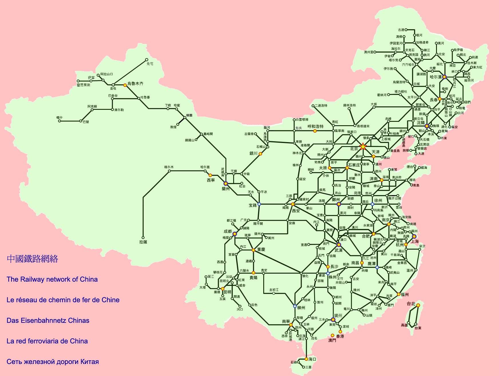
Figure 1. Chinese Railway Map
Dijkstra’s algorithm
Dijkstra’s algorithm is an algorithm used for computing the minimum distance and path between two points in a network of points. It was conceived by computer scientist Edsger W. Dijkstra in 1956 [1]. It can be explained better by graph and table as shown below:
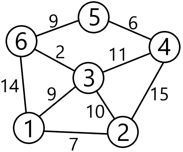
Figure 2. Dijkstra Concept Illustration Diagram
In terms of this project, the number inside the circle in Figure 2 represents the railway station. The lines connecting two circles represent the railways and the number aside the lines is the distance of that railway. For example, to get from station 1 to station 4, there are multiple choices. The dijkstra’s algorithm which is explained below with tables will help us find the shortest distance from station 1 to station 4.
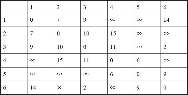
Table 1. Initial Setup with Parameters from Figure 2
The starting point is 1. To get the minimum distance between 1 and each of the remaining stations, row 1 would be updated several times according to Table 1. Firstly, from point 1 to point 1 itself, the distance is 0 which is definitely the shortest. So, we won’t update this value any more. Then we find the minimum value in row 1 and its corresponding point which is 7 connecting to point 2. We won’t update the value 7 any more for we can make sure it’s the shortest distance from point 1 to point 2. Next, given the determined shortest distance from point 1 to point 2, row 2 would be regarded as the next starting point. If the distance of row 1 column x is larger than the sum of distances of row 1 column 2 and row 2 column x, row 1 column x would be updated to be the sum of distances. x can be from any number in {3,4,5,6}. In this way, row 1 is updated to be:
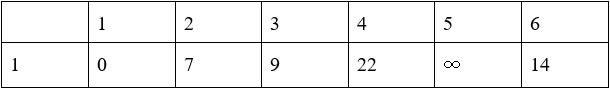
Table 2. Row 1 Updated from Row 2
Now, besides the fixed value 0 and 7, the minimum value in row 1 is 9 which is corresponding to point 3. We will set the value 9 fixed for we can make sure it’s the shortest distance from point 1 to point 3. Next, row 1 would be updated from row 3 for the shortest distance from point 1 to point 3 has just been determined. If the distance of row 1 column x is larger than the sum of distances of row 1 column 3 and row 3 column x, row 1 column x would be updated to be the sum of distances. x can be from any number in {4,5,6}. Row 1 is updated to be:
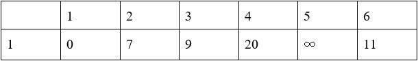
Table 3. Row 1 Updated from Row 3
With same method, update row 1 from row 6, row 4 and row 5 respectively. The result is shown below:
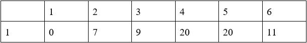
Table 4. Shortest distance from point 1 to other points
At this stage, row 1 represents the minimum distance between node 1 and each of the other nodes.
Existing Products
The function performed by this program is similar as using Google Map or Baidu map searching in the Transit mode.
Program/Hardware Design
Software Details
Map Display
The Chinese railway map as Figure 1 shows was firstly modified by MATLAB in order to be displayed in VGA. The modified picture is shown below.
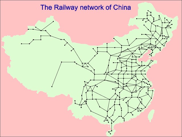
Figure 3. Modified Chinese Railway Network
We convert this picture from .jpg to .bmp then we can read its pixel information easily using C code. We have a function in our code called map_display to be in charge of displaying this map. The map_display function will read this .bmp file in sequence. After reading the header information like the height and width of this picture, the B, G, R value of each pixel will be read. We incorporate the separate RGB value into the 16-bit format then we can use the VGA_pixel function provided by Bruce to draw this picture on VGA screen. The relevant code is shown below.
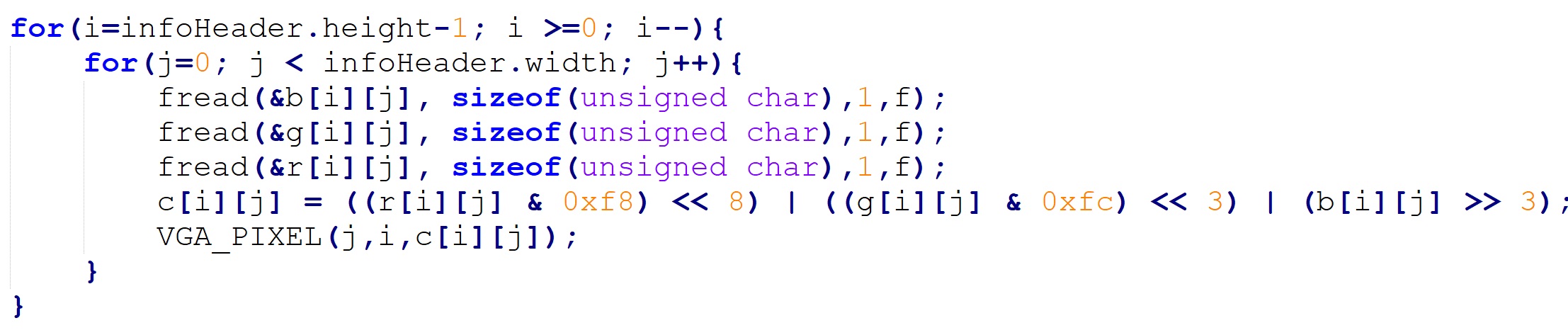
Figure 4. VGA display
Dijkstra Function
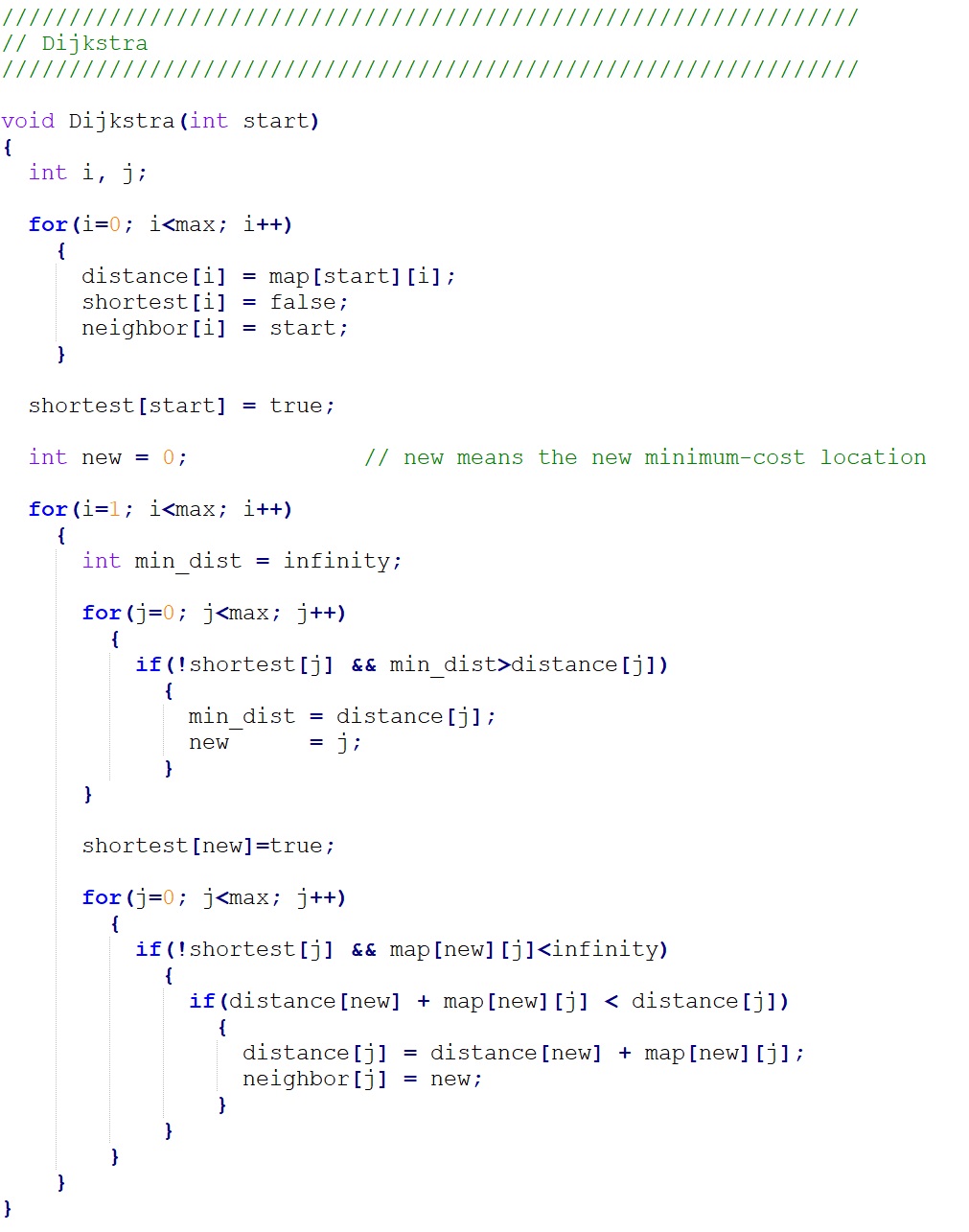
Figure 5. Dijkstra function
The Dijkstra function is the core function in our code.
Once the user selects the start location, the start location will be transmitted to this function as the parameter “start”. The parameter “max” indicates the total number of stations in our map, the 304. The parameter “infinity” is a huge number which indicates there’s no connection between two stations.
There are three important arrays in the Dijkstra function: distance, shortest, and neighbor. The distance array stores the distance from start location to any other station which will be updated 303 times to make each cell the shortest one. The shortest array indicates whether the corresponding distance is the shortest. If one cell of the shortest array is true, then the corresponding distance won’t be updated. The neighbor array is helpful later to find the shortest route from the start location to the destination. It stores the station from which the corresponding distance will be updated.
In the first “for loop” in our code, we will initialize the value of the three arrays. The second “for loop” will loop 303 times to get the shortest distance from start location to any other station. In the second “for loop”, there are two sub “for loop”s. In the first sub “for loop”, the minimum distance among all the unfixed distance will be found and in the second sub “for loop” the distance and neighbor array will be updated.
Min_path Function
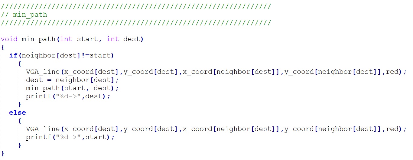
Figure 6. Min-path function
The min_path function is a recursive function which helps us display the shortest route information from start location to the destination. Once the Dijkstra function is done, we get a neighbor array with useful information. In each of its cell, there stores the station from which the corresponding distance has been updated to the shortest one. We transmitted our selected start location and destination to the min_path function as the parameter start and dest. And then use those two parameter and the neighbor array to display the shortest route.
Hardware Details
After the implementation of Dijkstra algorithm in C code, we will implement it on FPGA.
First, we need to implement 304*304 storage cell on FPGA board to store the map information as Table 1 shows. As 304*304 is a big number, we will implement these storage cells with M10K blocks. We choose to implement 304 M10K block in our design, each of which has 304 storage cells, representing a column in Table 1. Then we set a variable “counter” to be used as the address of all the memory blocks. In this way, we can read or write 304 storage cells, all in the same row as Table 1 shows, in the same cycle. Here we need to notice that the M10K block takes two cycles for read. We need to follow a certain style to implement the M10K block and use generate to implement it by 304 times. The relevant code is shown below. For the three important arrays mentioned above in the Program details, we just use register files to implement them for each of them just has 304 storage cells.
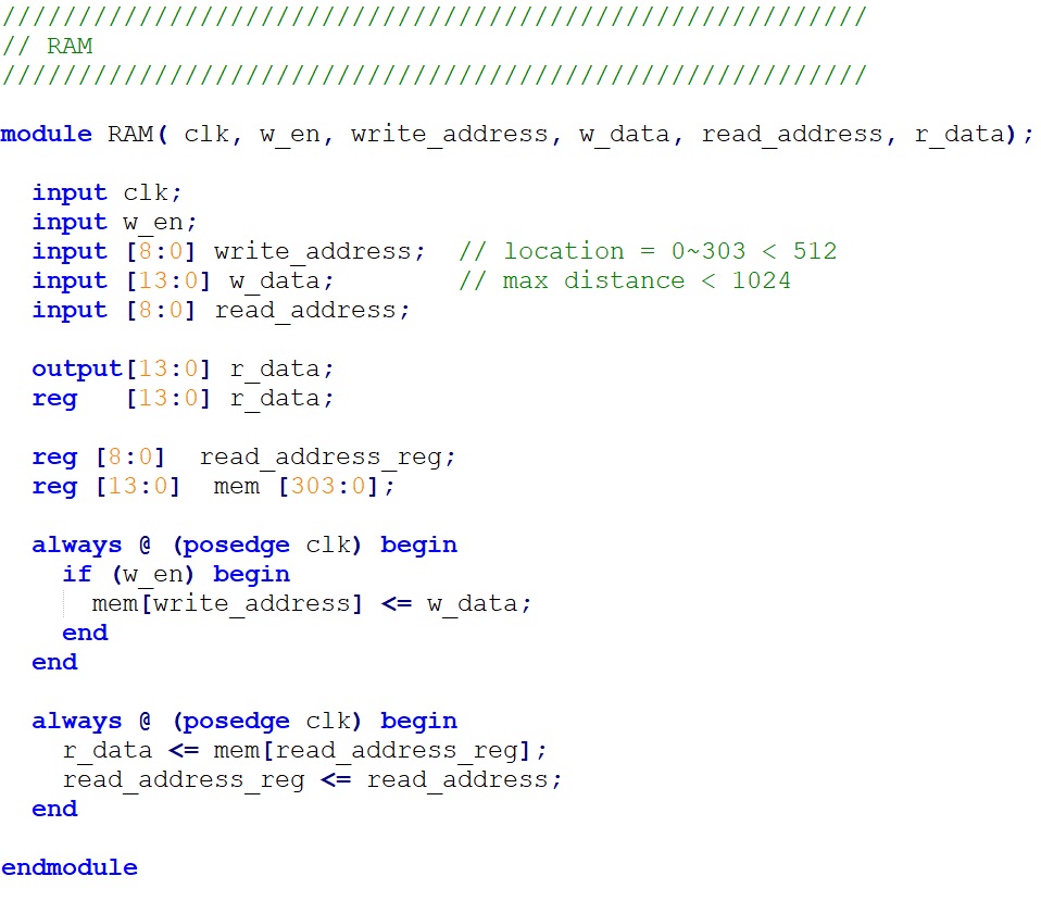
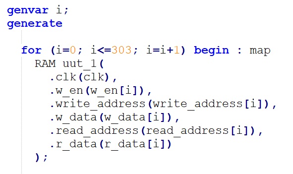
Figure 7. Memory
The implementation of Dijkstra function on FPGA is based on the FSM design structure. The state transition always block is shown below.
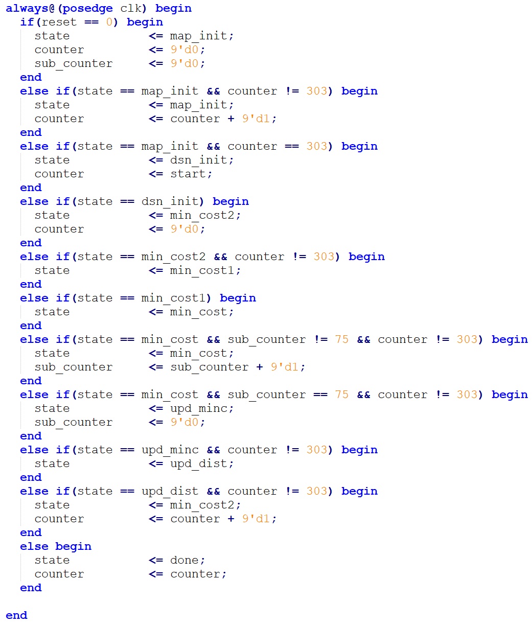
Figure 8. FSM
In the state map_init, we will initialize the map memory we’ve just implemented, which takes 304 cycles to move to the next state. In the C code, this step takes 304*304 loops to initialize the map by reading a data from a .txt file in each loop which will take a long time. Therefore, we won’t include this time period for initialization in our later comparison between FPGA and HPS only. Otherwise we may see that our FPGA implementation is 70 times faster than HPS which is just an illusion.
In the state dsn_init, we will initialize the distance registerfile, shortest registerfile and the neighbor registerfile which is corresponding to the distance array, shortest array and the neighbor array in the C code, respectively.
Naturally, after the dsn_init state we want to move forward to the state min_cost in which we will find the minimum distance among all the unfixed distance like what we wrote in C code. However, as M10K block takes two cycle to read, we set two more state min_cost2, min_cost1 as an interval before we move into min_cost to wait the distance registerfile, shortest registerfile and the neighbor registerfile complete their initialization.
The state min_cost will take 76 cycles because as we discussed in the High level design, we implemented four 2-input comparator in our design so we need 76 cycles to get the minimum distance out of 304 distance. In C code this step takes 304 loops to get the minimum distance.
Then we move to the state upd_minc in which we will update the shortest array.
Next, we will move to the state upd_dist in which we will update the distance registerfile and the neighbor registerfile in one cycle. Our 304 M10k block each representing a column in Table 1 allows us to achieve such a quick update. In C code, this step takes 304 loops, updating a storage cell in distance array and neighbor array in each loop.
Then we will move back to the state min_cost2 until we repeat such flow by 303 times, which is corresponding to the second loop in C code. We can’t decrease the iteration times here and once the flow iterates 303 times, we will move to the state done.
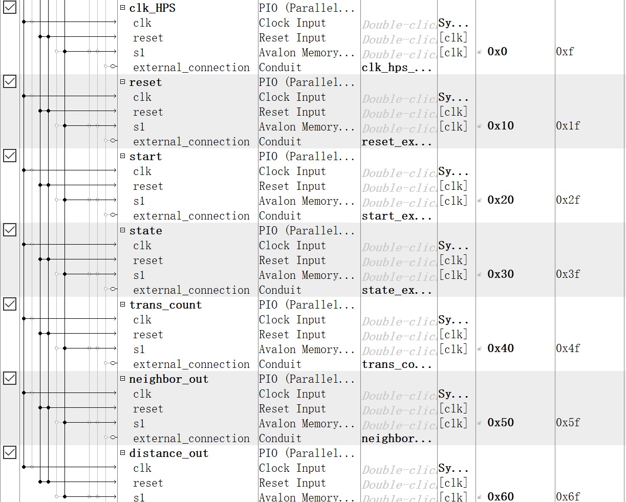
Figure 9. Qsys
Once we get to the state done, we need to transmit the data in distance registerfile and neighbor registerfile back to the HPS. Therefore, we need to add some parallel I/O port in Qsys to build the connection between FPGA and HPS. The added Parallel I/O ports are shown above.
clk_HPS is the clock signal generated by HPS to drive the circuit on FPGA.
reset is also generated by HPS to control the reset time on FPGA.
start is an output of HPS to transmit the start location to FPGA.
state is an input of HPS which tells HPS when the FPGA moves to the state done.
neighbor_out and distance out are input of HPS which transmit the data in distance registerfile and neighbor registerfile to HPS serially.
trans_count will count 304 times to make the distance_out and neighbot_out complete their transmission.