FPGA Knn Recognition

kNN Overview

Machine Learning Algorithms:

Machine learning algorithms are divided into two categories: lazy and eager learning. Lazy learning algorithms consist of storing training data and calculating some result once new incoming data is received whereas eager training consists of pre-calculating an algorithm and using this for new incoming data. These can be further divided as supervised or unsupervised learning. Supervised learning requires the testing data to have been pre-classified whereas unsupervised doesn't.

Classification:

Classification is a supervised and commonly lazy method of learning. In general, there are two stages of this process: training and classification. The training stage consists of feeding pre-classified data into the model to develop a dataset which can be used during the classification stage. The classification stage consists of feeding new, unclassified data into the trained model and attempting to fit a new label to it. Popular classification algorithms include Naive Bayes, Support Vector Machines, and also Nearest Neighbors algorithms.

kNN Algorithm:

Our project focuses on implementing the k-Nearest Neighbor (kNN) algorithm. As with most classifiers, the algorithm takes in pre-classified data during the training stage. During the classification stage, the algorithm determines the distances between the new test data with the entire training set and looks at the k, a user-defined constant, closest neighbors and selects the highest occurring neighbor. In other words, we can split the algorithm into three main stages: distance calculation, sorting, and selection.

kNN Algorithm

High Level Design:

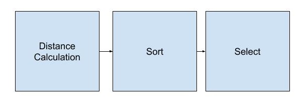
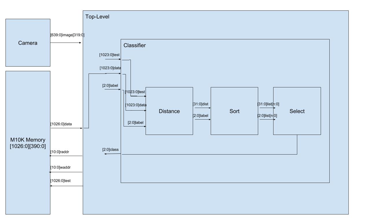
The design of the kNN hardware consists of three main blocks: distance calculator, sorter, and selector.

Pipeline:

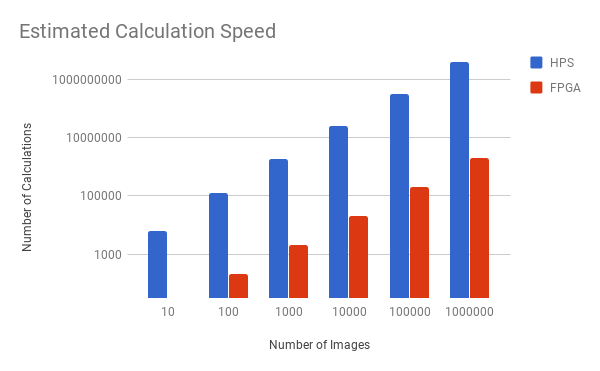
Our classifier pipeline consists of a single-cycle distance calculator, a single-cycle sorter, and a k-cycle selector. In other words, the classifier receives a block of classified data from our training set along with a new block of test data and calculates the distance while placing it in a re-sorted list in one cycle. The algorithm performs this calculation for each of the blocks of data in the training set so it takes n cycles to calculate the distance between the new block of test data with n blocks of classified data in our training set. Afterwards, our pipeline takes k cycles to look at the k closest neighbors in our sorted list and outputs this as the new label for our test block.

Figure: Pipeline

This kNN pipeline has been specialized for image recognition and designed specifically for how we are encoding images. As described above, we have decided to encode images into 64, 16 bit words which act as an intensity histogram. Mapping this to our hardware, our distance calculator involves summing the differences between each of the 64 words for the block of trained data and the new block of test data. Our sort consists of taking in the calculated distance and maintaining a sorted list for all of the blocks of trained data. And our selector looks at the first k elements in the sorted list and outputs the highest one.

Figure: Block Diagram

Distance:

The distance calculator went through many iterations of design. The first design involved a 12-cycle pipeline to reduce the total number of adders used and hopefully allow more parallelization. After some initial testing of this design, we moved to a 1-cycle combinational design as the additional logical units used to handle state wound up taking more space than expected. The final distance module simple takes in the 64, 16 bit words for both the trained data and test data, both represented as 1024 bit inputs, and performs 64 subtractions in parallel followed by 60 additions.

Sort:

The sorting algorithm went through numerous iterations as well. The original design involved a two cycle / two stage sort of each data piece. The first cycle was meant to decide where the new data will go, and what data had to be displaced in order to accommodate the new data, and the second cycle was to settle all of the data in the correct places. We challenged ourselves to improve the design. The main motivations behind this challenge were that the data was fed to the sorter in series and our main goal was to show hardware acceleration of an existing algorithm. The final implementation sorted the data that was incoming to the sorting module in a single cycle, deciding both where the new data belongs and how to displace the previous data on the same cycle.

The final implementation of the sorter was inspired in part by our implementation of the drum synthesizer in one of the previous labs. The drum synthesizer had cells that represented nodes on the drum and had access to the information about their neighboring cells that was necessary to determine their next value. Similarly, the sorter consisted of an array of bucket modules that were generated to correctly sort the data as it came in. The buckets had information about the new data coming in, the status and value of themselves, and the status and the data in the bucket above.

Each bucket module had a bucket_data register to store the data, and a bucket_full register to keep track of the status (full or empty). Both these registers were connected to the outputs of the bucket module. The inputs of the bucket module were clock, reset, and enable, as well as new_data input representing the data coming in, and above_data and above_full to keep track of the data and status of the above bucket respectively.

On each clock cycle the bucket would decide which data to store. Each bucket was initially (and on reset) set to be empty and have a stored value of "0". If the above bucket was empty, the bucket did not store anything, and stayed empty. The top most bucket had the above_full input hard-wired to full, and the above_data input hard-wired to 0 (the smallest possible Euclidean distance). If the current bucket was empty, the above bucket was full and the above bucket data was not greater than the new data, the bucket stored the new data. If the current bucket data was greater than the new data and the above bucket data was not, the bucket also stored the new data. However, if at any point the above bucket data was greater than the new data, the current bucket always stored the above bucket data.

Select:

The selecting module was the bottle neck of the entire process. After all the data was sorted the selector had to look at the top k pieces of data and choose which tag was the most common among them. In other words the selector would choose the tag that was represented the most often among the images that had the least distance from the given image - choosing the mode of k nearest neighbors. The selector waited for the sorter to finish, iterated through each of the top k data pieces once, and then, during the following cycle, decided which tag among them appeared most often. We also improved the design by having the selector not only output the selection, but also output confidence in the form of how many matching data sets were among the top k.

Figure: Percent Accuracy of Select

Results of the Design

Performance and speed-up:

The final design saw a very large increase in terms of performance. The first iteration of the design involved using PIO pins to pass down the image histogram to the HPS which would then run the kNN classifier. In terms of performance calculation, for each image this design needs to iterate through a 64 element array and perform a subtraction, negation, and a rolling addition followed by a memory write. In other words, we will have two main for loops which will compile down to at least 512 ARM instructions (not counting jumps and control flow logic). After this, we have to sort the array which is O(nlogn) in respect to the number of images, in terms of instructions this can vary but is at least the number of elements multiplied by its log. Lastly, it will have to reiterate through and calculate the closest neighbor which is O(k) with respect to the chosen k. In other words, we will take at least (512+896)*n+k cycles where n is the number of faces stored in memory and k is the selected k.

In comparison, the FPGA calculates the distance and maintains the sorted list in 1 cycle and then takes k cycles to select. In other words we take a bounded n+k cycles where n is the number of images and k is selected. Because of this, we predicted a speed-up of around 1000x in terms of raw cycles and a couple hundred accounting for the slower clock on the FPGA. Getting the official results, we saw that the classifier took 9680 cycles at 800000 MHz on the HPS for 10 images with a value of 10 for k whereas the FPGA took 20 cycles for the same test but at the FPGA's 50000 MHz clock. Running 100 images, the number of cycles for the HPS increased exponentially to 6500000 cycles where as the FPGA took 110 cycles. In other words we see an exponential increase in terms of computation time for the HPS while the FPGA increases linearly. With the relatively small data size of 100, we saw a speed-up of 3600x.

Figure: Classifier Speed

In terms of accuracy, the model performs as expected. In other words, the accuracy increases exponentially based on how well you train your model. The first iteration of our design allowed a maximum of 100 images to be stored. For facial recognition, we saw that having around 25 images for each face warranted near perfect results assuming background images stayed relatively similar. The final compiled design had a maximum of 300 allowed stored models which would allow for a much higher accuracy. As a benchmark it seems at least 25 saved images for each classification lends to around 99% accuracy rate.

Figure: Accuracy of Classifier

There were really no safety considerations other than following general proper coding procedure to ensure no unexpected or undefined behavior. In terms of usage, we saw that the user interface was relatively easy to follow. We had Key 3 capture a new image and assign the label as Switch 6, Switch 5, Switch 4. Key 2 would try to classify a new image capture. And Key 0 acted as a reset. We had many peers try our project and all of them responded that it was very intuitive.

Classifier:

The original design of the distance calculator consisted of a 12 cycle pipelined distance calculation. This was to prevent large fan-out from instantiating 64 subtractors as well as 60 adders and having these all be connected for a 1-cycle computation. The original design had a slightly more complicated pipeline where 12 of these 12 cycle pipelined distance calculators would be instantiated and there would be an arbiter used to decide which distance calculator to use at each cycle. Ultimately, these two designs would lead to similar throughput (assuming the same level of parallelization) while saving on a couple potential adders and also drastically decreasing fan-out. However, the secondary design ultimately proved to be much better. The logic utilization (total ALMs) used for the first design was 6230/32070 and the number of registers used was 9826. For this new design, we had a logic utilization of 3230/32070 and the number of registers decreased to 6237. It also met timing for the given FPGA's clock.

Sorter and Selector:

Both the sorter and the selector went through multiple iterations. The trickiest part was to balance the complexity of a single cycle sorter and keeping the design "light-weight" to conserve ALMs in case they were needed for other parts of the project. Many iterations of the sorter bucket modules had more inputs from other buckets and contained multiple registers. Having registers in the design always increased the number of necessary cycles and made the design more convoluted. The final solution to sorting was quite elegant and used as few interconnections between bucket modules as possible. The design of the selector was less involved, but, due to the cumbersome nature of iterators in Verilolg, took quite a bit of time to test. As part of testing the selector module, we were checking how many of the top k neighbors were matched to the chosen result. We decided to keep that information as something we "bubbled up" to the user to see how close the match was, and potentially make decision about having to train the algorithm more.

The resulting design for sorting and selecting was far faster in hardware than its software counterparts, as was intended. Even the best sorting algorithms have a complexity O(nlogn) while ours had the worst-case timing of exactly n. The sorting was completed in n cycles, where n was the size of the training set. The decision regarding classifying the image was reached in k+1 cycles, where k was the chosen number of nearest neighbors to look at.

Appendix A

The group approves this report for inclusion on the course website.

The group approves the video for inclusion on the course YouTube channel.