High Frequency Trader
Steven Lambert, William Barkoff, and Ryan Kolm
We attempted to create a high frequency trader (HFT) to be used in the stock market. While the impact of this design may seem only monetary in worth, this project allows us to show the benefit of hardware acceleration, parallelization, and networking that can be done on the Cyclone V and DE1-SoC pair.
Rationale
High frequency trading has become a very large part of investment in the United States and around the world. According to a 2016 Deutsche Bank report, high frequency trading accounts for about 50% of trade volume in the United States, and 35% in Europe. Initially, high frequency trading focused on finding arbitrages, where fast trades could effectively guarantee a profit; however, as market infrastructure began to match that of the trading industry, these arbitrages became fewer, shorter, and harder to exploit. High frequency trading then pivoted to a prediction based model, where high frequency traders attempt to predict what will happen to the stock in a very small amount of time, and use that prediction to perform a trade.
Many high frequency trading firms are employing FPGAs in an attempt to speed up their trading algorithms, making this a good, real word example of FPGA use in industry.
Project Sources
These sources were used as a basis for our ideas and implementation. For some of the underlying math, we cite the work by Jacob Loveless, Sasha Stoikov, and Rolf Waeber, and for some of the initial logic ideas, we cite the work by Arévalo, Andrés & Nino, Jaime & Hernandez, German & Sandoval, Javier.
- Jacob Loveless, Sasha Stoikov, and Rolf Waeber. 2013. Online Algorithms in High-frequency Trading: The challenges faced by competing HFT algorithms. Queue 11, 8 (August 2013), 30–41. https://doi.org/10.1145/2523426.2534976
- Arévalo, Andrés & Nino, Jaime & Hernandez, German & Sandoval, Javier. (2016). High-Frequency Trading Strategy Based on Deep Neural Networks. 9773. 424-436. https://doi.org/10.1007/978-3-319-42297-8_40.
Project Structure
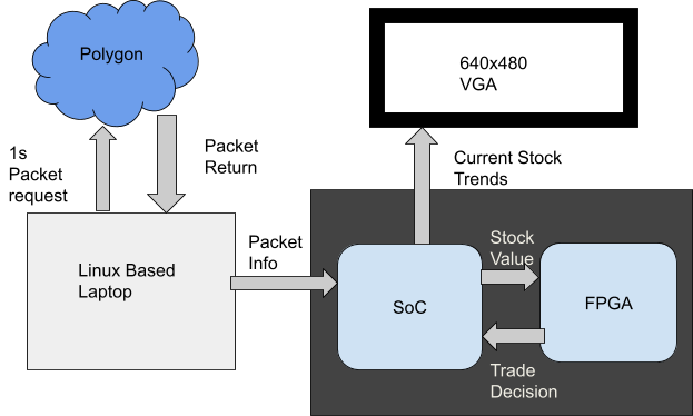
The figure above describes our design at a very high level. To get real time data, we used polygon.io which offers a real-time stock data API. For our intent and purposes, we used the starter subscription that provided us current stock data that was delayed 15 minutes to real time. As we are only simulating our trader, this delay is acceptable for we can simulate it as the real situation. We can only request windows of 1 second through this API which limits our operating speed. However, we can show the response time of our hardware to show the fastest response time it can achieve.
The SoC is running a network monitor to receive the stock packets from the laptop via ethernet. The SoC will decipher the packet and transmit the information to the FPGA via PIO ports. It will also use the data to graph current stock trends on a connected 640x480 VGA for user viewing. The FPGA will take the current data and perform a trader analysis that is described in the hardware design. Once the analysis is completed, it returns trade information back to the SoC that describes the decision for current stock trend and the “strength” of that decision. “Strength” meaning the amount to trade if choosing to buy or sell. The SoC uses that information to update the changes in the system's portfolio which is available to the user via serial output. At the start of the simulation, we give each running stock $10,000 and run 10 stocks in parallel to one another.
In order to get the data from the internet to the FPGA, we need to use another computer. Cornell IT's security policy prevents us from connecting the FPGA to the network outside the 10-space. In order to get the data, we wrote a Go program that connected to Polygon's websocket API that received data aggregated over each second on 10 stocks. We then connected the FPGA to the computer with an ethernet cable and assigned it a link-local address (specified in RFC 3927). This means that the computer and FPGA can talk to each other, but the FPGA cannot talk to any other devices on the network.
The program took the websocket packets and constructed new packets, which it then forwarded over UDP to the FPGA. Each packet contained information on one stock, and was 4 bytes long. The top 5 bits indicated the symbol of the stock, represented as an integer, and the bottom 27 bytes represented the value of the stock in fixed-point notation. One of these packets was sent each time a stock received an update from the Polygon API.
We initially implemented the software with TCP; however, UDP would allow for a performance increase if stock data was provided more frequently. There is however a greater chance that packets would arrive corrupted or out of order; however, with the direct ethernet connection between the laptop and FPGA, this chance is still very low, and an acceptable trade off.
As we were not able to move the entirety of the trader solely onto the FPGA, we sacrificed some execution time. The network interface was implemented on the SoC instead of the FPGA which limits our design to the speed of the PIOs. Since the SoC is not connected to the internet directly for security reasons, we are bottle necked at that transaction as well. Due to the dependency of digital signal processing (DSP) blocks, we can only parallelize up to 81 stocks, which is well above our testing desires. We are able to utilize only 1 DSP per stock because of the money management on the HPS side and by hardsetting an alpha parameter allowing our design to use shifts instead of another DSP, this is described further in the math section.
HPS
Our HPS code is relatively simple. It operates in two threads. The first thread reads
incoming stock data from stdin and writes it to the FPGA. It also reads
trades from the FPGA, and keeps track of the balance and holdings. The second thread
updates the VGA display with incoming stock information and portfolio information, which
arrives from the internet and from the FPGA. Network data is piped into stdio with the
netcat command.
Verilog
Our trading algorithm uses an exponentially weighted moving average and variance in order to make a decision to buy, sell, or hold a given stock. For the math behind both of these, we referred to “Online Algorithms in High-frequency Trading: The challenges faced by competing HFT algorithms” by Loveless, Stoikov, and Waeber. In this paper, the authors describe exponential algorithms for both average and variance that both only require one input per iteration and only one value stored in memory between iterations. This helps to keep each instantiation of the average and variance computation lightweight, which in turn allows us to be more efficient with the resources available on the FPGA such as DSPs. The idea was that if we kept this computation efficient then we could compute for more stocks on the FPGA. The calculation done for the moving average is as follows:
\[X^{AVG}_{0,\alpha} = X_0\]
\[X^{AVT}_{t,\alpha} = (1 - \alpha) X_t + \alpha X^{AVG}_{t-1,\alpha}\]
Before any math is done, the average is initialized to be the value of the first input, \(X_0\). After this, each subsequent average is a sum of some portion of the new input and some portion of the old average. The weight placed on the old average, \(\alpha\), is the smoothing factor and determines how much emphasis the computation places on old data versus new data. In other words, can be thought as of a low-pass filter on new data. In our design, \(\alpha\) is hard-set to a value of \(0.94\). To minimize the number of DSP blocks in use, multiplication with as an operand is optimized to be a shift operation instead. To get \(0.94\) times another operand, we simply take the other operand and subtract it by itself shifted to the right four times. To get \(0.06\) times a different operand (\(1-\alpha\)), we shift the operand by four to the right.
To calculate variance, we follow a format similar to the one we used to calculate the moving average. Instead of initializing the starting value to the first input, the first variance value is set to equal one. After that, the second equation of the following two is used:
\[V_0 = 1\]
\[V_{t,\alpha} = (1 - \alpha)(X_t - X^{AVG}_{t,\alpha})^2 + \alpha V_{t-1,\alpha}\]
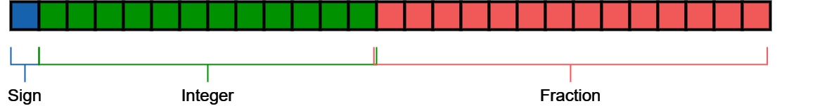
Because of our shift optimization for \(\alpha\) as discussed before, the module that calculates average and variance only uses one DSP block per instantiation. The only case where actual signed multiplication is necessary is for calculating the square in the variance equation above. As an aside, because the DSP blocks take in operands of 27 bits in length, we opted to use a fixed point format of 13 integer bits (one for sign) and 14 fractional bits. This afforded us enough precision and enough numerical range to properly capture stock prices.
Trading Algorithm
To implement the trader, we made a K-Nearest Neighbors algorithm (KNN). The algorithm's intention is to catch corners in the current trend for a stock. Due to the speed operation, we are using the prior 60 seconds as the training group for comparison The algorithm operates as follows:
Collect 60 seconds and thus 60 instances of stock value at start up. During that collection, take a simple 1 instance Manhattan distance between the current price and the opening price at the start of 60 seconds.If the distance is negative and is below the lowest distance in the set, set that recorded distance as the lowest for the set. If the distance is positive and is above the highest distance in the set, set that recorded distance as the highest in the set. After 60 instances, make trade decisions based on the current price inflows. If the distance of the new price is negative in relation to the price 60 seconds ago but is above the lowest, buy the stock. If the distance is positive in relation to the price 60 seconds ago but is below the highest, sell the stock. If neither is the case, hold the stock. Add the new price to the set and remove the oldest price recorded. Set the new oldest price as the sample price for the distance.
Our original algorithm was close to the flow diagram in the paper by Arévalo, Andrés & Nino, Jaime & Hernandez, German & Sandoval, Javier. However, their design used much more of a deep-learning algorithm which was beyond our scope. Thus we abstracted away but may still have some similarities to. This KNN algorithm described above was then implemented into hardware on the FPGA.
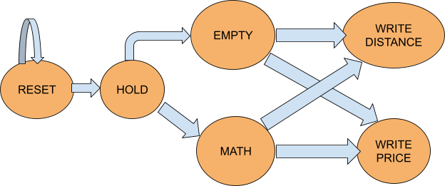
To explain a bit of the complexity happening in the trader, we made the forward based state machine above which does not show recursion in the state machine. At reset, the system sets all the used registers to zero. This includes distances, prices, trade choice, memory addresses, and state transition variables. Following reset, the machine holds on trades until there is a price change that is inputted by a pio. After a price change, the machine checks to see if the simulation has just begun or not. If it has, then the memory is deemed empty and needs to be written to, thus populating the 60 neighbors in the algorithm. For memory, we are using M10K blocks structured by 256 x 32 blocks (this is based on example 12-16 here). We write both distance and price to memory. In the order seen in the memory, the first index is the price for that specific time instance and the second index is the distance from the 60 second starting price. This pair allocation is followed for all price instances. While populating the initial 60 prices, find the lowest and highest prices in comparison to the sample price and record these distances in a register.
Once the first 60 prices are collected, the algorithm can move onto decisions in the math state. When a new price enters, compare it to the sample price. If the distance of the new price is negative in relation to the price 60 seconds ago but is above the lowest, buy the stock. If the distance is positive in relation to the price 60 seconds ago but is below the highest, sell the stock. If neither is the case, hold the stock. Add the new price to the set and remove the oldest price recorded. Set the new oldest price as the sample price for the distance. Write the price and its distance to memory. This is all contained in the KNN module in the hardware system.
After the trader makes a choice to buy or sell the stock, how does it choose the amount? As we struggled setting exact values, we came up with using percentages. If the trader gives a 0 for a trade, then it is a very weak decision and thus trades 0% of the stock/allowance. If the trader gives a 10 for a trade, then it is a very strong decision and thus trades 100% of the stock/allowance. The middle range fills in by degrees of 10%. Now what determines this percentage. Look at the example below:

This example shows the case for selling. The solid line is the current price trend and the dashed line is the predicted average price for the average unit. We found that at corner changes, the avenge will either transition above or below the trend. This can be used in determining the proximity to a corner change. The example shows that a weak sell occurs when the averager is below the trend as the averager is now expecting the price to fall therefore indicating a higher price rise, and the intersection has passed. A strong sell occurs when the averager is above the trend line as the averager is expecting the price to rise and therefore indicating a lower price, and the intersection has not come yet. This is reversed for buying. Once the trade is determined as being either strong or weak, we can utilize the variation in the price to the averager to determine accuracy of the current guess. We chose the following thresholds for accuracy after manualing analyzing some trends:
- If variation > 450: low accuracy
- Otherwise, if variation > 250: low-medium accuracy
- Otherwise, if variation > 100: medium accuracy
- Otherwise, if variation > 50: high-medium accuracy
- Otherwise: high accuracy
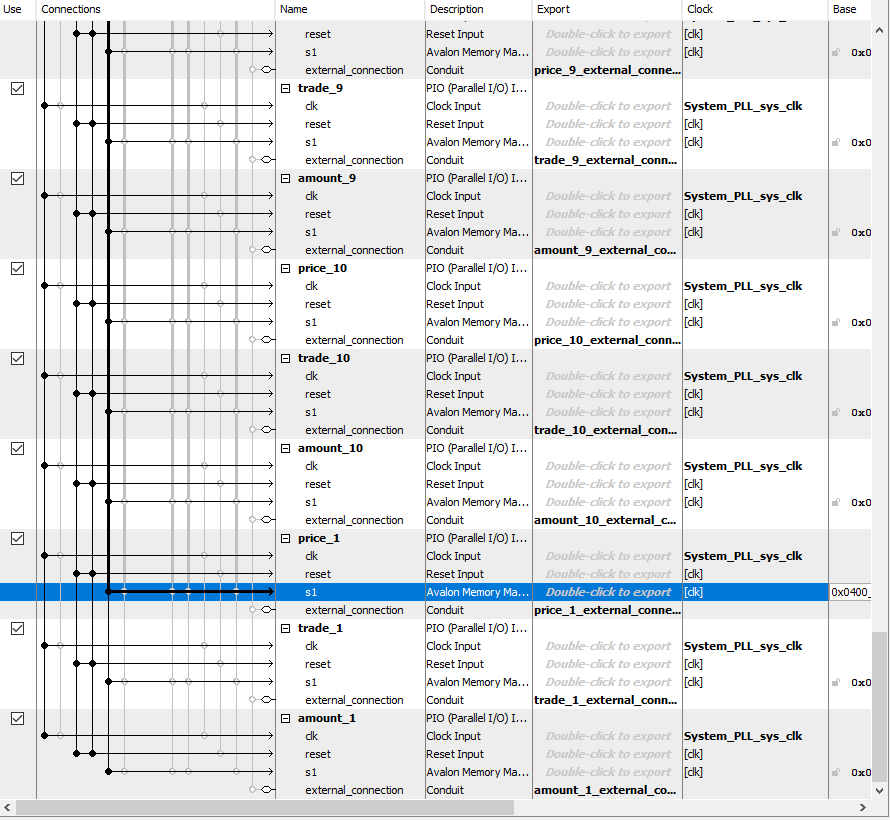
In the final system, we set up 10 parallel traders to perform the described analysis. Each trader was connected to three PIO pins, one pin for the price, one for the trade choice, and one for the amount to move. We also had a VGA subsystem which was utilized by the SoC. This system was derived from example code from the ece5760 course site listed here. These connections are shown in our Qsys. A snippet of our Qsys is shown below.
Other design elements that we scrapped
Initial trading algorithm
We initially tried to use a similar logic flow as the one described in the second referenced paper above. However, we quickly realized that this path was not ideal for the type of flow we were trying to achieve. Our machine needs to evaluate the current flow of data and not the historical trend as that paper was trying to achieve. We also did not have as rigorous of a ML model making it not a great flow for our design. Therefore, we opted to use the algorithm above.
Wallet management on FPGA
We tried to implement the wallet management system on the FPGA to attempt to make the entire system on the FPGA. This proved to be much more troublesome than anticipated. Without using more DSP or making a time consuming divider, the states were becoming very long and complicated. Then when testing, the math would not be correct. It was elected to move this to the SoC to save us on time and resource intensity. This also allows execution time on the FPGA to be much faster than if it had to waste cycles doing division.
Network interface on FPGA
Initially, we planned on implementing the network interface on the FPGA; however, we anticipated numerous issues when sharing the ethernet interface between the FPGA and the HPS. We decided that we would attempt to implement the network interface on the FPGA at the end if we had time, and unfortunately we ran out of time to do so.
Results
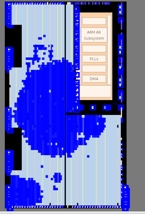
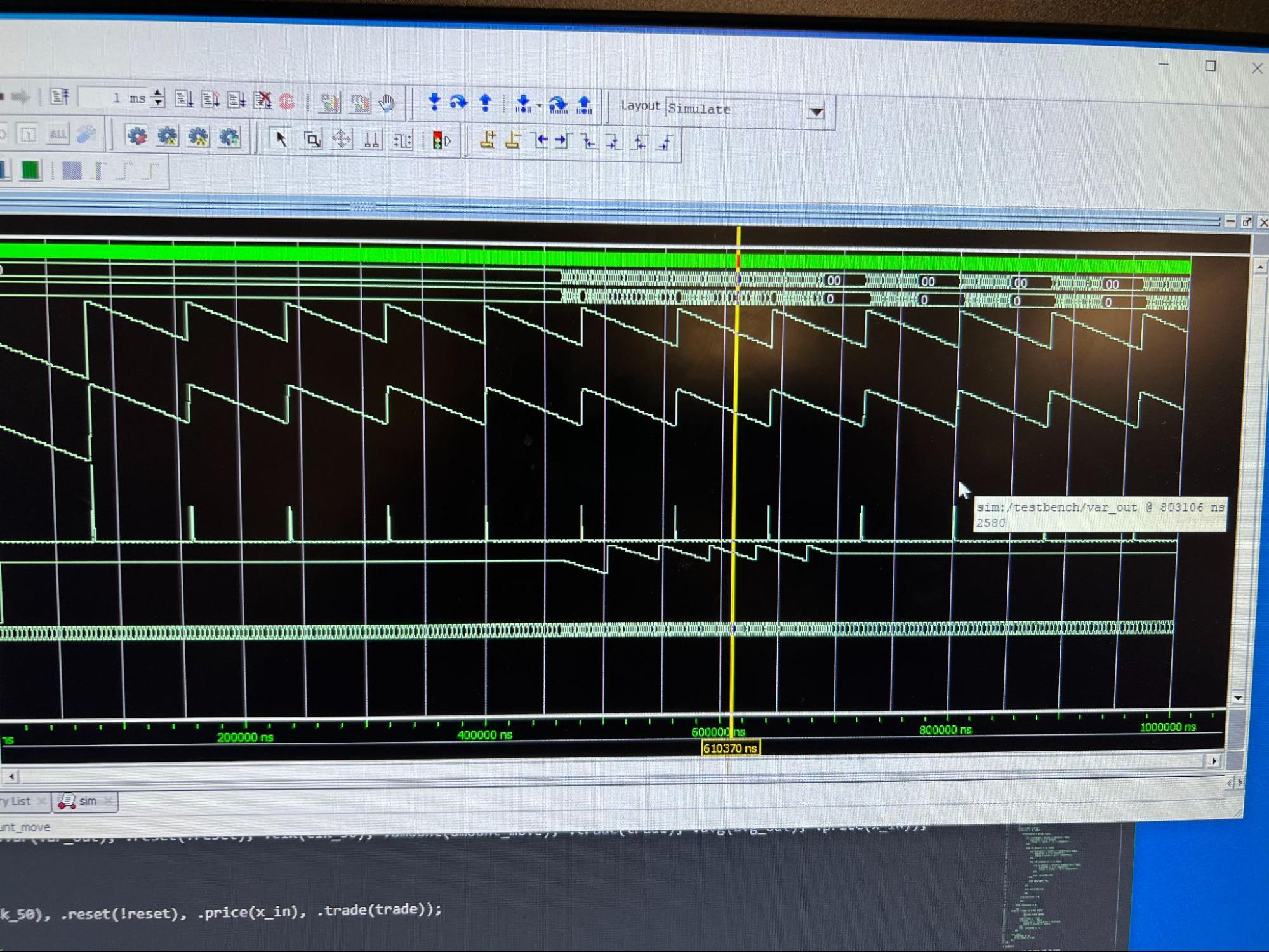
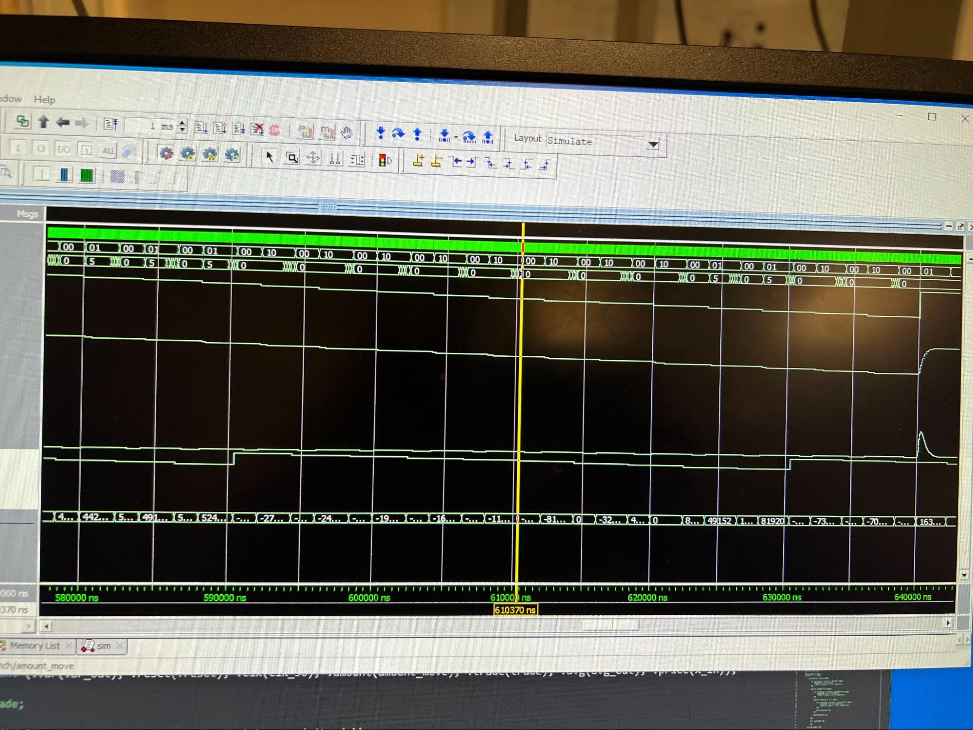
The figures below show a lot of the results of our design. The overall chip utilization is shown. While there is high density, there are still a lot of spare resources. This was expected as we were not parallelizing to our theoretical max for testing. If we pushed our design to handle more stocks, we would expect this utilization to spike. The following image shows the operation of our trader for a period of time. You can see the rapid decisions and trades it is deciding on. The image after that blows up on an instance in particular to show the time to commit to a decision. As we have set our design to hold the lowest and highest for the past prices, it can actually decide to buy or sell at a given price in one clock cycle, which for us is about 20 ns since we are operating at 50Mhz. It then takes about 62-64 clock cycles to update the KNN parameters. Therefore, it has a fast reaction to change but a slower refractory period to adjust. However, this would limit our design's speed to an absolute fastest of 1.3us with given variability, if there is no delay in transmission. For obvious reasons that is not the case but proves the swiftness of execution on the FPGA.
After analyzing the simulation and different simulation runs, we found that the algorithm was performing rather well. At occurrences of sharp corners, the trader would buy at the low points and sell at the high points with strong strengths. We did see odd occurrences of buy or selling on linear trends, but these were deemed weak as we hoped. After a few trades of weakness, the algorithm swapped to opposing trade which kind of catches its mistake. This was the best outcome we could have hoped for, granted we were not able to test directly to real-time data due to complication in the SoC and FPGA communication. These simulation results proved rather successful, and we argue that this algorithm has roughly 60-70% accuracy in corner detection which is about 10% higher than other algorithms in this field. As for safety in the design, it's risky as any other investment. It has the possibility to lose all of the money it has allotted to it when it is mispredicted. Though, if we were able to finish testing to verify further, I am inclined to give it some real money to see how it would perform. As for usability, one would need some minor code knowledge to set stock parameters and provide income, but outside that, it is pretty much autonomous.
Conclusions
Our design worked well. We were overall happy with the performance of the design on simulations, and we were happy that we were able to receive stock data on the FPGA. Unfortunately, due to an issue with the memory-mapping and the avalon bus, we were unable to test our design end-to-end. Next time, we would likely begin implementing the memory mapping sooner, so that we have more time to debug it.
Our design conformed to standards well. With the exception of boilerplate from earlier in the semester, we did not reuse any code. We do not foresee any patent or trademark issues.
Appendices
Appendix A: Permissions
- The group approves this report for inclusion on the course website.
- The group approves the video for inclusion on the course youtube channel.
Appendix B: Work Distribution
- Steven Lambert worked on the KNN trader algorithm and the strength decision. Both are encased in the KNN module and the amount module respectively.
- Ryan Kolm worked on the math for average and variance calculation, and wrote the Verilog for these computations
- Will Barkoff worked on the network interfaces. He wrote the HPS code, as well as the code on the networked computer that transmitted the stock data over UDP.
Appendix C: Code Listings
- Fiance.c (misspelling intentional)
- vga.c
- vga.h
- DE1_SoC_Computer.v