
Guitar effects have been around for many decades now and have become an integral part of the music we listen to. The basic design of guitar effects amplifiers has stagnated somewhat since its inception. Even new digital effects are based on analog designs. This project takes a different stance on how to create guitar effects by performing distortion in frequency domain, rather than by dealing with physical devices and their nonlinear characteristics. The goals are to use a frequency framework to make designs similar to existing effects, as well as to create completely new sounds.
Quick Music Background:
This section will relate some technical aspects of signal processing to their musical counterparts. This may be skipped, and does not pertain to my project in particular.
We hear according to frequency. However, we do not hear linearly. We hear the same pitch (an octave) as a doubling in frequency. In Western music we spread 12 equally spaced tones across each octave. As we hear by frequency, the interesting aspect of any amplifier is in how it affects the pitch of an input signal. If we were to consider a distorted sinusoid (of great importance, as a plucked guitar string is very close to a sinusoid, at least for a small time window), we could relate every new frequency to the fundamental frequency of that wave. According to the Fourier Theory, we know that every introduced frequency will be a multiple of this fundamental frequency (as the resulting signal will be periodic with the same period). This is interesting, as it contrasts the exponential nature of how we hear pitch. These introduced pitches will not necessarily be all of the same pitch. We assume that the amplitude of each introduced pitch diminishes as frequency increases (as is the case, considering the worst clipping possible would be a square-wave, which has diminishing amplitudes). Thus, we are only really interested in the first fifteen or so multiples of the fundamental frequency. These frequencies, their relation to the fundamental frequency, and their musical relationships are tabulated below. For relationship, I successively divide the frequency by 2 until it is between 1 and 2, which represents the frequency of the same pitch in the octave of our fundamental frequency.
| Multiple of FF | Relative Frequency | Musical Relationship (in Semitones) | Musical Relationship (Interval) |
| 1 | 1 | 0 | |
| 2 | 1 | 0 | |
| 3 | 1.5 | 7.0195 | 5th |
| 4 | 1 | 0 | |
| 5 | 1.25 | 3.8631 | Major 3rd |
| 6 | 1.5 | 7.0195 | 5th |
| 7 | 1.75 | 9.68827 | Minor 7th/Major 6th |
| 8 | 1 | 0 | |
| 9 | 1.125 | 2.0391 | Major 2nd |
| 10 | 1.25 | 3.8631 | Major 3rd |
| 11 | 1.375 | 5.513 | Sharp 4th/flat tritone |
The musical relationship can be attained by taking the log of the frequency relationship to the power of 1.059463, which is the 12th root of 2. This spacing is that of 1 semitone – the smallest interval in Western music.
What this shows is most of the low harmonics contain musically related frequencies. As the harmonics increase, the relationships become more and more dissonant. The 7th harmonic is the first to sound out of place, not being a true musical relationship. Later, the 11th harmonic introduces an interval that is almost directly in between the common intervals of Western music. While it sounds fairly pleasant on its own, it will likely stand out when in the context of music. This trend only continues as higher harmonics are considered.
First we see that some of the lower harmonics contain pleasant musical intervals:
Major 3rd
5th Harmonic
As you may be able to hear, the harmonics are not true musical tones. The 5th harmonic in this case is very close to a major 3rd, but it slightly flat. Even so, in the context of music it is close enough to sound pleasant.
The higher harmonics, however, are less musically related:
7th harmonic (between major 6th and minor 7th)
11th harmonic (between 4th and tritone)
both of these intervals sound somewhat dissonant. In music, this effect will be increased, as both fall between true musical intervals.
Given this tool, we can characterize how an amplifier should sound by considering the frequencies it introduces to a signal relative to its fundamental frequency.
Background and Motive:
Many kinds of guitar effects exist. Some of the earliest effects were the result of overdriven amplifiers, resulting in a “clipped” signal. This clipped signal introduces new frequencies to the signal, often resulting in an interesting sound. Other effects exist, such as time delays (echo, chorus, reverb, etc.), but in this context I refer to guitar effects as distortion of a signal with no time delays.
Effects in this sense came about when amplifiers were overdriven. The signal is clipped, introducing new frequencies. What frequencies are introduced depends both on the signal and the amplifier. The two broadest classifications of amplifiers are solid-state and vacuum tube (valve) amplifiers. Vacuum tubes are commonly characterized by “soft clipping.” That is, when the signal distorts, it does so gradually, instead of reaching a hard cut off at some amplitude. Solid-state amps, on the other hand, typically display “hard clipping” where the signal abruptly cuts off. This is demonstrated below, with transfer curves and the result of distorting a sine wave with these functions:
|
The importance of this distortion is the new frequency content. The input sine wave has only one frequency, but the output will have many more. A fourier analysis would reveal the specific frequencies in the signal. We can see, however, that the signals (especially the hard clipped) approach square waves, containing only odd harmonics. It is also important to note that a square wave contains very high frequencies (infinitely high, in fact) even if they diminish quickly. These two properties (odd harmonics and high frequencies) characterize the hard clipping amplifier. The fact that only odd harmonics are present means that some possible frequencies are missing. Tube amplifiers commonly contain these frequencies and are considered to have a “fuller” sound. Of the even harmonics, the 2nd, 4th, and 8th harmonics contain only the same pitch (although in higher octaves) as the fundamental frequency. This leaves the 6th and 10th harmonics, which sound as a major 5th and major 3rd, respectively. Any higher harmonics will likely drop off quickly enough to have little effect on how pleasing it sounds. We will explore how these even harmonics are introduced below.
The other property of hard clipping amplifiers is high frequency content. As I discuss in the music background, high frequencies are likely to be musically unrelated to the fundamental frequency. This makes them sound very dissonant. You experience this when you hear a very harsh distortion that sounds like white noise. This is something we would like to avoid.
Vacuum tubes, unlike most solid-state amplifiers, have a special trait – their transfer curve is asymmetric. The soft clipping curve shown above does not exactly capture that of a real vacuum tube, which would look more like the one below:
 |
As you can see, the output signal is asymmetric. If the DC value is discarded, this can be viewed as a close to a square wave with a changed duty cycle. It will contain even harmonics. Solid-state amplifiers have been created with asymmetric transfer curves. However, they still clip harder than vacuum tube amplifiers and aside from their low price do not offer any new, useful sounds.
This has been the basis of most distortion effects to this point. Digital amplifiers have been introduced, but they are still based on the governing equations of transistor and valve amplifiers.
As we hear according to frequency, it makes sense to pursue distortion effects directly in frequency domain. From our consideration of classical amplifiers, we know that the perfect distortion amp should contain those low harmonics that are musically related to the fundamental frequency and exclude all high harmonics. This is not possible with old amplifier techniques, but should be possible in frequency domain.
There is one major difference that this sort of amplifier will produce. To this point we have considered only sinusoids, which are a good approximation of a single guitar string. When multiple strings are played, or a more complicated signal (a voice, for example) is introduced, our amplifier will act differently. Normal distortion effects will produce frequencies according to how it clips the entire signal. They may have arbitrary relationships to the frequency content on the input signal. My amplifier design allows the output signal frequencies to always be related to the input frequencies. It, however, makes it more difficult to introduce frequencies as a function of the existence of multiple frequencies in a signal, as classical amplifiers do.
Design Theory- FFT based design:
As the goal of my project is to process a signal in frequency domain, I started out by creating a simple pitch shifter, which could later be expanded upon. I shifted the pitch using a short time fft, shifting the magnitude of each bin to the bin representing twice the frequency.
There were three parameters to take into consideration when shifting audio samples: window size/shape, overlap, and phases. I arbitrarily kept the phase of each bin the same as the input. This shouldn’t matter so long as the window length is short enough that all frequencies are heard as pitches, not as timing information. For example, if the window period gets longer than about 100ms the timing of the audio sample will change. As far as the window length, it must be long enough so that the lowest expected frequency in the sample can be detected by the fft. So the window must be as long as the period of our lowest frequency. In the case of a guitar effects processor, we expect the lowest frequency to usually be low E – a frequency of 82.4 Hz. We must also account for a low D, as guitars are frequently tuned with the low string tuned down a whole step, to “drop D tuning.” Low D has a frequency of 73.4 Hz. Accordingly, our window needs to be at least 14 ms. At a sampling frequency of 44100 Hz, this corresponds to about 617 samples per window.
The final considerations are the window shape and overlap. Because I will be computing a short time ifft to create the distorted signal, there will be aliasing between the frames. We can reduce this by overlapping the frames and windowing them with a triangle, Gaussian, or some similar form. Using a triangle window with an overlap of 2 works well, as does a higher overlap with a Gaussian window.
With these parameters settled, audio can be shifted with decent results. Note that for a signal that sounds good, a window size of at least 4096 is required.
each of these audio samples is of a C-major scale on guitar. They are shifted one octave higher using a gaussian window 3 standard deviations wide and an overlap of 4. Varying window length is shown, displaying the necessity for a large window.
Original Recording
Window = 2048
Window = 8192
With a working shifter, harmonics can be introduced to the signal. The process is very similar to the pitch shifter, with different shift magnitudes mixed into the signal. The links below contain a distorted Cscale with varying window lengths. In addition, a series of chords are provided in their original and distorted forms.
The following recordings are distorted with a mix of .8 of the original recording, .2 of the first harmonic, .5 of the third, .2 of the 4th, .3 of the 5th, and .2 of the sixth.
C-scale, window = 2048
C-scale, window = 4096
C-scale, window = 8192
Guitar Chords
Distorted Chords window = 4096, overlap = 4
An interesting effect is evident in these samples: the shifted pitches occur at a different time than their original pitch. This occurs because the window is too large. With a window of 4096/8192 samples, frequencies as low as 10 Hz will be detected. Humans cannot hear these frequencies at pitches. They are so low that manifest themselves as the shape of the audio signal, not the pitches that we hear. When these frequencies are shifted, the shape of the audio signal is changed, which is not what we intended. On the other hand, if the window is any smaller, low pitches will sound garbled, even though our fft should properly detect these frequencies.
The chords, however, still have decent locality in time. It is a more stationary signal than the scale, so a larger window is acceptable in this case.
The problem is that we do not have good frequency resolution for low octaves. If we use 1024 samples per window, our fundamental frequency would be 43 Hz, enough to detect the lowest frequencies we would use. However, the first octave, from 73.4 Hz to 146.8 Hz would have only 2 frequency bins. The number of bins per octave grows exponentially, doubling for each successive octave. For higher octaves, we will even use too many bins, to the point that we are wasting processing power.
As such, we need a method of exponentially spacing the frequency bins so that each octave has the same frequency resolution. My first attempt to do so is to make a filter bank and obtain a frequency representation of a signal by passing the signal through a series of bandpass filters, calculating the power in that range, and attributing all of that power to the center frequency of the bandpass. A shifted signal can then be created by direct digital synthesis.
Filter Based Design
Using filters is rather different from the previous approach in many ways. ffts are so simple in that it is unnecessary to specify frequency bins. We now need to worry ourselves with the details filtering the signal to obtain an accurate, resynthesizable frequency representation. As a first attempt, I started with a similar function declaration: y = distort(x, window, overlap)
The first goal was to take in a signal, filter it, determine the energy content at each frequency, and synthesize a signal, hopefully sounding the same as the original. Window and overlap work in the same way as they did for the fft-based distort function. However, I eventually decided to stick with just using triangle shaped windows and an overlap of 2. Because we are directly synthesizing the signal, the phase will be continuous between frames. Thus, an overlap of 2 with a triangle window will linearly interpolate the amplitude of each frequency between frames. For windows that are small relative to how quickly an audio signal changes, this will be sufficient. (filter/distort.m. See Code Appendix)
The first new design parameter introduced was a vector of frequencies, f. From this vector the filter bank would be created. I started by forming 2nd order band pass Butterworth filters using adjacent frequencies as the 3 dB cutoffs. The power observed in each filter would be synthesized as the center frequency of the filter. The choice of 2nd order Butterworth filters was motivated by the fact that I knew I could implement these in Verilog when building the final design.
Having a mechanism for designing filters, I would need to specify the frequency spacing. Naturally, the spacing should place more filters in lower octaves and fewer filters in higher octaves. This is, after all, the reason for using a filter bank instead of an fft. The question still remains how many filters should be spaced per octave. Perhaps an easier question to reason about is: how many filters should be spaced between 2 adjacent musical notes. While the closest 2 formal musical notes are to each other is 1 half step (a factor of 1.059463), filters will have to be placed closer than this to account for frequencies that occur in between, such as with guitar bends, harmonics, or any other sounds.
The selection of frequency boundaries is not an easy one, and is central to a proper design. Once the filters are set, they can operate on the signal, at which point an RMS value can be computed to determine the peak amplitude to synthesize for each frequency. Each frequency is synthesized, being sure to keep the phases equal between frames, the result is windowed and added to an output vector.
It should be noted that such a design is very difficult to work with in Matlab. To process a 3 second sample with 20-40 filters can take from 5-10 seconds. You can then imagine that a longer audio sample with filters spaced throughout the audio spectrum would take several minutes to process. To alleviate these issues, I made a series of sine-based samples to process. The advantage of these is that they are relatively narrow banded and will require fewer filters to process. The samples include: a pure sine wave, a linear fm sweep from 1 tone to a higher tone, alternating tones, a linear fm sweep back and forth between 2 tones, and a sine wave fm sweep between 2 tones. A function generates each of these, so that I can quickly modify what frequencies are used, how far apart they are, how long the samples are, and how many times they oscillate (for those that do). Generally, I used high A (880 Hz) and high Bb (about 932 Hz). This way I could address just a small half step of frequencies, hopefully answering the question of how many frequency bins should be placed per half step. Samples are provided below (filter/sinesamples.m. See Code Appendix):
| no modulation | linear up | linear down | sigmoid up | sigmoid down | sine | |
| pure sine |  |
|
|
|
|
|
| linear fm sweep | |
|
|
|
|
|
| alternating tones | |
|
|
|
|
|
| linear sweep periodic | |
|
|
|
|
|
| sine sweep | |
|
|
|
|
|
Next I created a script to automate the processing of multiple samples at once so that I could quickly compare different configurations (filter/filtersinesamples.m. See Code Appendix). At this point the only parameters I could change were the frequencies and window length, but more would follow. I soon found my first problem with this design: Butterworth filters, while simple and easy to deal with, are very flat at 2nd order. This is not a problem for other applications such as voice frequency where the frequencies of concern are spaced far away from each other and are discontinuous. In music, however, we cannot afford to disregard any frequency- the filters must be placed continuously. This means that the filters must overlap. In my first design the filters ‘touch’ at their 3dB points. This means that when a pure sine wave exists in the middle of a filter, the adjacent filter will still see power. In fact, it will see enough power to synthesize a wave of aslmost half the original’s amplitude. Filters that are farther away will also see power as it tails off. These other synthesized frequencies create beats in the output that make it sound incredibly muddled. Aside from deciding on the spacing of frequency bins, the rest of the design focuses on isolating frequencies from neighboring filters. After a long time experimenting, the following solutions were introduced:
One of the most obvious ways to increase the cutoff rate of a filter is to increase its order. By increasing the order of the filter to 4 or 6 we can increasingly isolate each filter. Increasing the order of the filter carries a large computation penalty as the number of multiplies and additions is proportional to the order. It is unlikely that any higher order solution would fit on the fpgas at my disposal.
Along with order, we can also change the cutoff rate of a filter by changing its type. Originally we used a Butterworth, but we can also use a Chebyshev filter. Chebyshev filters have a very high cutoff rate at the expense of ripples inside the pass band. It remains a good option to test. For this to be effecting we would need to increase the order, as 2nd order Chebyshev filters have no ripple, and are thus very similar to Butterworth filters.
Previously, filters were aligned at their 3dB points. If the filters are designed to be ‘tighter’, adjacent frequency bins will not notice as much power for a given frequency. This was implemented by defining separation to be a number between 0 and 1. For a given set of boundary frequencies, the filter is centered on the average of the 2 frequencies. The width of the filter is defined by the difference of those frequencies multiplied by separation. The disadvantage to this approach is that there will be some dead space between each bin where neither filter observes the full power of the signal. In this case both will be synthesized to some extent.
These 3 parameters can be observed graphically below (filter/drawPeakResponse.m. See Code Appendix):
All plots are shown with 5 filters logrithmically spaced between 840 and 920 Hz. A red line is drawn at 880 Hz for convenience.
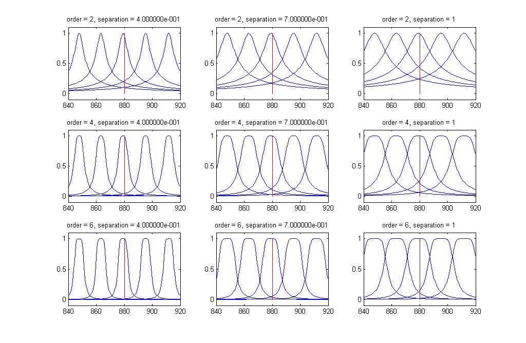


You can see that using higher order Chebyshev filters with carefully chosen separations the filters can be almost perfectly spaced and isolated. This offers a great improvement over the previous design. However, increasing the order is really not an option if we wish to implement the design in hardware. It is already uncertain if we will be able to fit enough filters simply to have enough frequency bins. Making each filter more expensive would be too expensive.
An alternative method is needed to remove frequencies with power observed from nearby frequencies. My first attempt came about when dealing with sine waves. I realized that the frequency bin that my signal was centered on would be synthesized with the full 1 peak. Those adjacent to it would synthesize a peak of .5, and it would slowly taper off after this. If I looked at each frequency and simply zeroed it if it was below some cutoff threshold, I would get the sine wave back as an output (aside from some transient time at the beginning where the filters outputs were moving to steady state). I defined a variable ‘c’ as the cutoff peak below which the frequency would be zeroed. In general this is a poor solution. A sample of soft music may be entirely cut out. This also does not address that the observed power is coming from adjacent frequencies.
I extended this idea by making c a vector of cutoff values. For each bin it would define what the power in adjacent bins would need to be relative to the power in itself for its output to be zeroed. For example, if c = [1 2 3] if the power in either bin directly adjacent to a specific bin was at least as large, the power in the next outside bins was twice as large, or the power in the bins outside those were 3 times as large, the output would be zeroed. This can be an effective technique of controlling erroneous frequencies being synthesized, but is difficult to design with. First of all, it is not immediately apparent how long this vector needs to be, in other words how far away from a frequency do we check. In addition, the actual cutoff values should be dependent on the specific filter and separation of filters. One also has to be careful to use somewhat conservative cutoffs to make sure that bins are not zeroed where some power actually exists.
Using these new design parameters: order, filter type, separation, and cutoff ‘c’, I should be able to find a working set to produce a good audio duplicate. The problem is in the number of configurations possible. Along with these, I still have the frequency vector and window length to specify. I modified my sample processing script to include these parameters. I found that I could process about 300 different configurations in about half an hour. Any more than 1500 configurations and my computer would run out of memory and essentially crash. This is too many configurations to be useful anyways. In general I selected 2-5 values for each parameter, listened to various outputs, and tried to find a combination that would work. This became very tedious, and I could not easily tell what changes were making the biggest impact.
A numerical method of comparing filters was necessary. My first instinct was that this could be done using a spectrogram, computing some norm between the spectrogram of the original signal and the processed one. However, spectrograms tend to use incredibly large amounts of memory, computing an fft for every window and then shifting the window by 1 sample. This resolution in time is also much greater than is useful. This being the case, I used an old script I wrote at the beginning of this project when I was analyzing a few audio samples: sparse spectrogram (filter/sparsespec.m. See Code Appendix). The sparse spectrogram computes ffts throughout an audio signal, but at large intervals. While it was designed for plotting spectrograms without computing more than was necessary, it will serve nicely as a metric for how similar two audio samples are. Using this script, I can look at how the norm changes with a variable, as demonstrated below:

In this sample, a cutoff is not used, resulting in many beat frequencies. As the number of filters increases, the sample becomes increasingly garbled.
It is important to note that I have assumed that when the norm is lower, the signal will sound better and be a better representation of the signal. This may not always be the case. However, very interesting trends can be observed. For example, I assumed that increasing the window length would generally lower the norm (improve the quality of the signal). As distort averages over a greater time it is more likely to notice the correct power per frequency bin. Of course, if the window length increases too much the signal will not change quickly enough. Observe one example of the effect window length has on the norm:


| Norm Mins | Norm Maxes | |||||
|---|---|---|---|---|---|---|
| 186 | 278 | 370 | 150 | 234 | 322 | |
| Set 1 | |
|
|
|
|
|
| Set 1 | |
|
|
|
|
|
As you listen for yourself you’ll likely notice that they do in fact sound much better. There are apparent beats, likely because I chose not to use a relative cutoff to remove errant frequencies, but you can still discern what the original signal was in half of them, whereas the other half sound very garbled. It should be noted that while the optimal window lengths are independent of the other parameters, they may be dependent on the actual signal. This is a very narrow band signal and there may be some relationship between 880Hz and this window length.
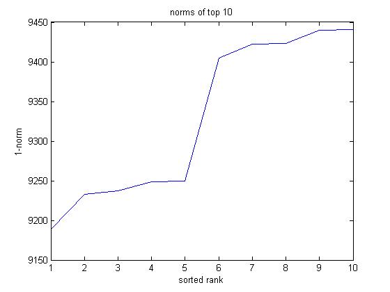
Knowing that this norm is a good metric for at least some parameters, I can use it to optimize my working set of parameters. If I sweep over a large enough number of values for each parameter and take the lowest norm, I should end up with a good method of finding the frequency representation of my signal. This takes a very long time, and if not programmed carefully can also take up too much memory. If any more parameters are added in the future, the space of possible parameters may become so large that an evolutionary algorithm would be more practical for optimizing the system. Run overnight, I found the following results (note that I omitted the relative cutoff. It is too difficult to design with):
(filter/filternorms.m. See Code Appendix)
window = [150 186 234 278 322 370]
separation = [.4 .6 .8 1]
order = [2 4 6]
ftype = {'b' 'c1' 'c3'}
logrithmically spaced frequencies from 860 to 1000 Hz. 10, 20, 30, and 40 frequencies.

| Rank | Audio | Window Length | Separation | Order | Filter Type | Number of Filters |
|---|---|---|---|---|---|---|
| 1 | |
186 | 1 | 4 | c3 | 10 |
| 2 | |
186 | 1 | 6 | b | 10 |
| 3 | |
186 | .8 | 4 | c1 | 10 |
| 4 | |
186 | .6 | 2 | c3 | 10 |
| 5 | |
186 | .6 | 2 | b | 10 |
| 6 | |
186 | .8 | 6 | b | 10 |
| 7 | |
278 | .6 | 2 | c3 | 10 |
| 8 | |
278 | .6 | 2 | b | 10 |
| 9 | |
186 | 1 | 6 | c1 | 10 |
| 10 | |
278 | .4 | 2 | c1 | 10 |
Looking at the data, most variables see a good range. However, all top 10 use only 10 frequency points (9 filters). This must be due to the fact that I did not use a relative cutoff, so more beat frequencies occur as more filters are introduced. I would expect that if I used a cutoff vector, a higher number of filters would be beneficial. We also see, interestingly, a dominant window length of 186, this being the smallest window length that performed well. This is a good thing, as a smaller window length means less delay in a real time device. All of the other parameters vary greatly across all their possible values. I was somewhat surprised to see so many 2nd order filters in this mix. They do in fact sound fairly good. If you listen for yourself, you’ll notice that all of the samples still sound a bit different from one another even if their norms are so similar. In my opinion, number 6 is the best, and also has the slowest beat frequencies.
While these still do not sound ideal, they demonstrate that it should be possible to obtain a good frequency representation from a filter bank. Additionally, this optimization shows that finding a good set of working parameters is rather unintuitive.
Once a good frequency representation of the signal is obtained, distorting it is simple. I specified a parameter in distort.m, synthfn, that handles all synthesis. It is a function handle that takes in a vector of frequencies, a vector of peaks (these 2 comprise the frequency representation of the frame), and a time vector which can be used to synthesize the sine waves. If any other information needs to be passed in, it should be curried into the function handle. Two examples are offered (filter/cleansynth.m, filter/synthfreqvec.m. See Code Appendix). Cleansynth simply synthesizes the signal as done before in distort. Synthfreqvector takes in an array in addition to the other parameters. The vector needs to be curried in before the function handle is sent to distort. This array should be nx2. The left column specifies relative frequencies, the right column relative peaks. This allows pitch shifting and mixing in of harmonics and other relative frequencies. The advantage of using filters and synthesizing manually is that now these relative frequencies do not have to be integer multiples, as in the fft based distortion. If we so choose, we can introduce perfect musical intervals into our signal. We can also shift down and by arbitrary amounts. The exams below demonstrate this function:
I use the parameters from the 6th ranked sample above.
| Original | Shift up by 1.5 | Shift down by 1.5 | Add harmonics (1st and 2nd) | Add low harmonics (.75) | Add musical major 3rd (x1.26) |
|
|
|
|
|
|
These do not sound musically appealing whatsoever due to the original signal being so bland, but they demonstrate the functionality of the destortion mechanism.
Conclusion
It is possible to create a decent distorting function in frequency domain. As I have shown, the limiting factor is one’s ability to obtain an accurate frequency representation of a signal. From that point synthesizing any desired signal is relatively simple.
Unfortunately, the computing power needed to obtain this representation is large. A huge number of filters are required, and it is better if they are higher order. This would require either building specialized hardware that can compute each filter in parallel, or using a computer with numerous processors, each running an independent thread for filtering different frequencies. Until I have access to an fpga with more floating point units or commodity processors with more cores, I won’t be able to build this. Given the rate that technology improves, however, it shouldn’t be too long.