3D-Biomorph
Project Advisor: Bruce Land
Li, Jen-Guan
E-mail: jgli@cs.cornell.edu
In the book "The Blind Watchmaker", Richard Dawkins[1] has described his journeys through a genetic cyberspace where he models the evolution of organisms he calls "Biomorphs" in 2D(dimensional) space. In this project, I tried to extend the Biomorphs to 3D(dimensional) space by using OpenGL graphics library. I call them 3D-Biormorphs in this report.
The original program in the book "The Blind Watchmaker" uses 16 genes to control the evolutions of 2D Biomorphs. In order to create the models for 3D-Biomorphs, I extend the number of genes from 16 to 25. There are 5 genes to control the depth extent, 1 gene to control the symmetric attribute of Z axis and 3 genes to control the colors of 3D-Biomorphs. Users can see the detail definitions in the Genetic Algorithm section of this report.
This project is a working prototype of mathematical models for 3D-Biomorphs. The goal of this project is to design and implement a working application that can see the manipulative evolutions controlled by 25 genes. In each new generation, there are 25 progenies shown in the same window. Each one has some minor changes in one of the 25 genes. Compared to their parent, there will be some differences between them. After 10 or 20 generations, users can easily find the changes among offspring and their original parent. Because each viewport(progeny) in the window maps to the changes of one fixed gene of its 25 genes, users can choose the same viewport as the parent of the next generation. After several generations, users can see the accumulative changes caused by the specific gene.
The goal of this program is to observe the evolutions controlled by 25 genes, so it provides some functions such as rotation, zoom in, and zoom out to help users to see the whole structure of the 3D-Biomorphs. The size of 3D-Biomorphs will automatically adjust to fit the size of the window. The following sections document some background information, the design and implementation, and how this project can be extended.
This project has three major parts -- the recursive mathematical algorithm, X-window and OpenGL programming.
I got the recursive mathematical algorithm from Richard Dawkins's book "The Blind Watchmaker"[1] and his paper "The Evolution of Evolvability"[2]. I introduce two improtant functions, tree and PlugIn, in the next section. Users can have a concept ual idea how these 3D-Biomorphs are bred. There are nither complex computation nor hard programming skills in this program. The point of this program is to observe the influences to the appearances of the 3D-Biomorphs.
X-window system is the standard window system designed by MIT for UNIX system about twenty years ago. In this program, most codes are traditional C language, but knowledge of creating window and writing event-driven programs is also required.
OpenGL is a high level graphics library provided SGI. It simplifies many complex operations such Z-Buffer, texture mapping and rotation into some very simple c library functions. Besides, it also provides very good resolutions in the results, so it has become the most widely used graphics library in the world. The other important issue of OpenGL library is that it provides the ability to draw 3D objects. This makes OpenGL an ideal tool in this program since 3D objects can be easily implemented.
Based on the above restrictions, I can only make sure that the program can be execute on the SGI workstations. RS/6000 is a possible choice to run this program, but users have to pay attention to two aspects. One is that the OpenGL library is correctly installed in the system. The other one is that the return value of rand function of standard library ranges from 0 to 32767 because I use the return values of this function to control the probability of genes' changes. Now this program can not be used on Windows 95 or Windows NT platforms. I will try to port the program by using Visual C++ and Windows NT. When this program can be available, I will put it on this web page.
Functions of the 25 Genes
This program breeds 3D-Biomorphs according to the definations of their genes. Users have to realize the function of each gene or they can not know what dose the program do and where is these 3D-Biomorphs come from. Each gene has different function in controlling the process of breeding. For example, gene 15 controls the number of segments of each 3D-Biomorph. If the value increases from 1 to 2. The 3D-Biomorph will become a two segments object instead of on segment. The following graph provides the detail describtion of these genes' function. While the program is running, users can see the effects of these genes in their corresponding viewport.
Figure 1. Diagram of ‘Chromosome’ indicating what each gene does
Gene 1-Gene 3
Horizontal Extent : These three genes control the horizontal extent of the 3D-Biomorphs. The larger the value of these gene are, the larger the 3D-Biomorphs in their horizontal extent. The initial value of these genes are controlled by a random number generator in the interval from -9 to 9. There are no limitations of their maximal or minimal values.
Gene 4-Gene 8
Vertical Extent : These five genes control the vertical extent of the 3D-Biomorphs. The larger the value of these gene are, the larger the 3D-Biomorphs in their vertical extent. The initial value of these genes are controlled by a random number generator in the interval from -9 to 9. There are no limitations of their maximal or minimal values.
Gene 9-Gene 13
Depth Extent : These five genes control the depth extent of the 3D-Biomorphs. The larger the value of these gene are, the larger the 3D-Biomorphs in their depth extent. The initial value of these genes are controlled by a random number generator in the interval from -9 to 9. There are no limitations of their maximal or minimal values.
Gene 14
Number of Branches : Gene 14 controls the starting value of length, the order of the recursive tree or in other words the number of branchings. The initial value is 1. The minimal value of this gene is also 1, but there is no limitation for the maximal value of this gene.
Gene 15
Number of Segments : Gene 15 controls the umber of segments of the 3D-Biomorphs. The initial value of this gene is 1. The minimal value of this gene is 1, but there is no limination for the maximal value of this gene.
Gene 16
Distance between Segments: Gene 16 controls the distance between each segment. The initial value of this gene is 10. The minimal value of this gene is 1, but there is no limination for the maximal value of this gene.
Gene 17
Bilateral Symmetry : Gene 17 controls the bilateral symmetric attribute of the 3D-Biomorphs. There are only two values, 'ON' and 'OFF', of this gene. The initial value of this gene in the program is 'ON'. I assume that all 3D-Biomorphs in this program are bilateral symmetry. That means the value of this gene will ramain on while this program is running.
Gene 18
Up-Down & Radial Symmetry : Gene 18 controls the up-down & radial symmetric attribute of the 3D-Biomorphs. There are only two values, 'ON' and 'OFF', of this gene. the initial value of this gene in the program is 'OFF'. While the program is running, viewport 18 will show the 3D-Biomorph with up-down symmetric attribute. Figure 14 is also a good example with bilateral and up-down symmetric attribute.
Gene 19
Front-Back Symmetry : Gene 19 controls the front-back symmetric attribute of the 3D-Biomorphs. There are only two values, 'ON' and 'OFF', of this gene. The initial value of this gene in this program is 'OFF', While the program is running, view port 19 will show the 3D-Biomorph with front-back symmetric attribute. Figure 15 is also a good example with bilateral and front-back symmetric attribute.
Gene 20
Scaling Factor : Gene 20 controls the scale with which all lines in a 3D-Biomorph are drawn. The larger the vale of Gene 20, the smaller the 3D-Biomorph. If you make a 3D-Biomorph small by means of Gene14, you can restore it to tis original appearance by proportionately increasing the magnitudes of Genes 1 to 13 and Gene 16. The initial value is 1. The minimal value is also 1, but there is no limination for the maximail value of this gene.
Gene 21
Mutation Size: Gene 21 controls the magnitude of each mutational step. If gene 21 has a small value, each mutational step will be relatively small in extent and vice versa. The ininial value of this gene is 1. The minimal value is also 1, but there is no limination for the maximail value of this gene.
Gene 22
Mutation Rate: Gene 22 controls the mutation rate, or probability of mutating, of all the genes. Most genes mutate at the full rate indicated by this gene. Others mutate at half the rate. There are only two values, 'ON' and 'OFF', for this gene. The initial value of this gene is 'ON'. 'ON' means other genes can mutate at the full rate. If the value is 'OFF", genes can only mutate at half the rate.
Gene 23
Color Red : This gene controls the intensity of red. Its value varies from 0.0 to 1.0. This inital value is determined by a random number generator.
Gene 24
Color Green : This gene controls the intensity of green. Its value varies from 0.0 to 1.0. This inital value is determined by a random number generator.
Gene 25
Color Blue : This gene controls the intensity of blue. Its value varies from 0.0 to 1.0. This inital value is determined by a random number generator.
Overview of this program
Figure 2 is an overview of the program. PlugIn and Tree are the most important functions in this program. PlugIn translates genes into variables needed by Tree. Tree is a recursive function to breed offspring. There are some introductions of these two functions in this report. Users can see the detail descriptions in Richard Dawkins's paper "The Evolution of Evolvability."[2]
Figure 2. Flow Chart of this Program
Genetic Recursive Algorithms for Breeding:
1.Create random initial population.
Step 1 initializes the value of variables used in this program. In the beginning state, all 3D-Biomorphs have the same status.
2. PlugIn
PlugIn translates genes into variables needed by Tree procedure. These variables have great influences on the position and size of the branchings of each 3D-Biomorph. There are detail explanation in Richard Dawkins's paper "The Evolution of Evolvability"[2]. The following procedure is originally from this paper, I modified it to fit the 3D environment. Actually, the corrreponging position for dy and dz are the same. Different mapping method might lead to different results. The only reason to use PlugIn function is to reduce the number of genes in controlling their extents. Users can see the mapping method in Table 1. There are 8 slots in each variable array, but there are only 3 or 5 genes to use. That is why we need a function to map the values of genes that control the directional extents into the proper slots.
| 0 | 1 | 2 | 3 | 4 | 5 | 6 | 7 | |
| Dx |
-gene[2] |
-gene[1] |
0 |
gene[1] |
gene[2] |
gene[3] |
0 |
-gene[3] |
| Dy | Gene[6] | Gene[5] | Gene[4] | gene[5] | gene[6] | gene[7] | Gene[8] | gene[7] |
| Dz | Gene[11] | Gene[10] | Gene[9] | gene[10] | gene[11] | gene[12] | Gene[13] | gene[12] |
Table 1. Mapping table among gene 1 to gene 13 and form dx, dy, dz arraies(arraies of variables).
procedure PlugIn (ThisGenotype: Genotype);
begin
order := gene[9];
dx[3] := gene[1]; dx[4] := gene2[2]; dx[5] := gene[3];
dx[1] := -dx[3]; dx[0] := -dx[4]; dx[2] := 0; dx[6] := 0; dx[7] := -dx[5];
dy[2] := gene[4]; dy[3] := gene[5]; dy[4] := gene[6]; dy[5] := gene[7]; dy[6] := gene[8];
dy[0] := dy[4]; dy[1] := dy[3]; dy[7] := dy[5];
dz[7] := gene[9]; dz[3] := gene[10]; dz[4] := gene[11]; dz[5] := gene[12]; dz[6] := gene[13];
dz[0] := dy[4]; dz[1] := dz[3]; dz[7] := dz[5];
end{PlugIn};
/* The call of Tree the follows:
Tree(Startx, Starty, Startx, order, Startdir, dx, dy, dz); */
3. Breed.
Tree is called with the arrays dx, dy and dz specifying the form of the tree, and the starting value of length specifying the number of branchings. Tree calls itself recursively with a progressively deceresing value of length until length reaches 0.
This procedure uses recursion to generate branches. The restriction was that children were only ‘allowed’ to be one mutation distant from their parents. In other words, only one gene was allowed to mutate at a time, and that gene was allowed to change it ‘value’ only by + 1 or -1. The point is adequately made if we restrict gene values to single figures, that is if we allow them to rage from -9 to 9. This is a simplified algorithm for breeding. In the actual program, random number generator is used to control the probability of mutation. This procedure is originally from Richard Dawkins's paper "The Evolution of Evolvability"[2]. I made a little modification of it to fit the 3D environment. It controls the direction and size of each line segment generated by the program.
procedure Tree (x, y, z, length, dir: integer; dx, dy, dz: array[0..7] of integer);
begin if dir < 0 then dir := dir + 8; if dir <= 8 then dir := dir -8;
xnew := x + length * dx[dir];
ynew := y + length * dy[dir];
znew := z + length * dz[dir];
push(x, y, z, xnew, ynew, znew); {store each line segment}
if length > 0 then { now follow the two recursive calls, drawing to left and right respectively}
begin
tree(xnew, ynew, znew, length - 1, dir - 1, dx, dy, dz){this initiates a series of inner calls}
tree(xnew, ynew, znew, length - 1, dir + 1, dx, dy, dz)
end
end{tree};
4. Draw the 3D-Biomorphs.
This step calls the OpenGL functions to draw the 3D-Biomorphs generated in step 3 and save them as individual display list.
5. Replace parent generation with children.
Step 5 show these new 3D-Biomorphs in the window for observation.
6. If end condition not satisfies, go to setp 7.
Step 6 tests the conditions specified by users. There are detail introduction of the conditions in the next section.
7. Select parent for next generation and repeat from step 2.
If the parent is selected in this step, go to setp to rebreed the next generation 3D-Biomorphs.
Data Structure Used in the Real Program:
1. Structure of 2 points to represent line segments.
A line segment consists of two points, so this program uses a sturcture to save their coordinate values of these two points and the pointer points to the next line segment. The pointer's value of the last line segment should be NULL.
struct lineseg {
GLfloat frontptx;
GLfloat frontpty;
GLfloat frontptz;
GLfloat endptx;
GLfloat endpty;
GLfloat endptz; /* GLfloat is a floating point data type defined by OpenGL library */
struct lineseg *nextline;
}; /* The real structure of one line segment */
typedef struct lineseg Myline; /* Define a new data type for line segments */
/* Stack (single linking list of line segments to represent one 3D object). */
Myline *startbiomorph[25]; /* Starting position of the the linking list */
Myline *currentbiomorph[25]; /* End position of the linking list */
2. Data structure used to represent genes and distance variables.
There are 25 genes used in this program. I use a structure to resprent the genes and variables used for the breeding process. I combine the genes with same data type of integer into arraies. If the gene need special data type such as Boolean or GLfloat to represent it, I use a single variable to represent it in this structure. There 25 progenies will be generate in each breeding cycle, so I use an array with 26 elements of this structure to store the information of these 3D-Biomorphs.
struct gene {
int gene[16];
Bool gene17; /* Bool is the type of Boolean */
Bool gene18;
Bool gene19;
int gene2021[2];
Bool gene22;
GLfloat gene23;
GLfloat gene24;
GLfloat gene25; /* GL float is a floating point data type provided by OpenGL library */
int dx[8];
int dy[8];
int dz[8];
int startdir;
};
typedef struct gene Mygene; /* New data type for genes */
Mygene offerspring[26];
F1
Terminate the program
F2
Initialize the program to the beginning state
Mouse Button 1
Select parent for breeding
Mouse Button 2
Switch the window from multiple 3D-Biomorph mode to single object mode
Mouse Button 3
Switch the window from single 3D-Biomorph mode to multiple object mode
Insert
Rotate 3 degrees by X axis
Home(only active in single object mode)
Rotate 3 degrees by y axis
Page Up(only active in single object mode)
Rotate 3 degrees by z axis
Delete(only active in single object mode)
Rotate -3 degrees by x axis
End(only active in single object mode)
Rotate -3 degrees by y axis
Page Down(only active in single object mode)
Rotate -3 degrees by z axis
Left Arrow(only active in single object mode)
Zoom in 10% of the original size
Right Arrow(only active in single object mode)
Zoom out 10% of the original size
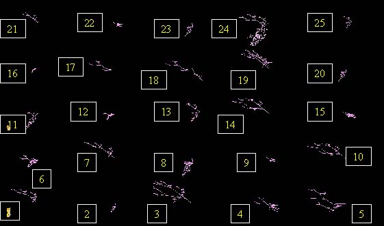
Figure 3
Multiple object mode with 25 3D-Biomorphs
1. Progeny with modification in gene1.
2. Progeny with modification in gene2.
3. Progeny with modification in gene3.
Gene 1 to gene 3 control the horizonal extent of the 3D-Biomorphs. Their appearance and size and size are changed due to the changes of these three genes.
4. Progeny with modification in gene4.
5. Progeny with modification in gene5.
6. Progeny with modification in gene6.
7. Progeny with modification in gene7.
8. Progeny with modification in gene8.
Gene 4 to gene 8 control the vertical extent of the 3D-Biomorphs. Their appearance and size and size are changed due to the changes of these five genes.
9. Progeny with modification in gene9.
10. Progeny with modification in gene10.
11. Progeny with modification in gene11.
12. Progeny with modification in gene12.
13. Progeny with modification in gene13.
Gene 9 to gene 13 control the depth extent of the 3D-Biomorphs. Their appearance and size and size are changed due to the change of these five genes.
14. The parent 3D-Biomorph.
15. Progeny with modification in gene15.
Gene 15 controls the number of segments of the 3D-Biomorph. I let this gene with 33% probabilities to plus or minus 1 in the breeding process. If changes happens, users can see the 3D-Biomorph with multiple segments.
16. Progeny with modification in gene16
Gene 16 controls the length between two segments. Because the change is very minor, it is hard to see the change in the appearance of the 3D-Biomorph.
17. Progeny with modification in gene17.
Gene 17 controls the 3D-Biomorph's symmetric attribute of X axis. In this program, I assume all 3D-Biomorphs are bilateral symmetry, so there are no modification of its genes. Theoretically, this 3D-Biomorph should has the same appearance with its parent(viewport 14), but it doesn't. The reason is that they started in different variables(the position in dx, dy, dz array) and different number of branches(the value of gene 14).
18. Progeny with modification in gene18.
19. Progeny with modification in gene19.
Gene 18 and gene 19 control the 3D-Biomorph's symmetric attribute of Y and Z axes. Their default values are Fault. That means the 3D-Biomorphs can have asymmetric appearance in their vertical and depth extents. If these two genes has any changes, the redraw function will modify their appearance into the symmetric form.
20. Progeny with modification in gene20.
Gene 20 controls the scale with which all lines in a 3D-Biomorph are drawn. The larger the value of Gene 20, the smaller the 3D-Biomorph.
21. Progeny with modification in gene21.
Gene 21 controls the magnitude of each mutational step. If Gene 21 has a small value, compared to gene 20, each mutational step will be relatively small in extent.
22. Progeny with modification in gene22.
Gene 22 controls the mutation rate, or probability of mutating, of all the genes. Most genes mutate at the full rate indicated by Gene16. Others mutate at half the rate.
23. Progeny with modification in gene23.
24. Progeny with modification in gene24.
25. Progeny with modification in gene25.
Gene 23 to gene 25 control the intensity of red, green and blue of 3D-Biomorphs. If there is any change in these three genes, users can see the different color from their parent in 3D-Biomorph 23 to 3D-Biomorph 25.
Figure 4
Single object mode of 3D-Biomorph 24
Figure 5
Zoom in 3D-Biomorph 24 in single object mode
Figure 6
Zoom out 3D-Biomorph 24 in single object mode
Figure 7
3D-Biomorph 24 rotate by X axis in single object mode
Figure 8
3D-Biomorph 24 rotate by Y axis in single object mode
Figure 9
3D-Biomorph 24 rotate by Z axis in single object mode
Figure 10
3D-Biomorph with single segment
Figure 11
3D-Biomorph with 2 segments
Figure 12
3D-Biomroph with 3 segments
Figure 13
3D-Biomorph with 4 segments
Figure 14
3D-Biomorph with symmetric attributes in X and Y axes
Figure 15
3D-Biomorph with symmetric attributes in X and Z axes
Figure 16
3D-Biomorph with symmetric attributes in X, Y and Y axes
Figure 17
3D-Biomorph rotates 0 degree by X axis
Figure 18
3D-Biomorph rotates 30 degrees by X axis
Figure 19
3D-Biomorph rotates 60 degrees by X axis
Figure 20
3D-Biomorph rotates 90 degrees by X axis
Figure 21
3D-Biomorph rotates 120 degrees by X axis
Figure 22
3D-Biomorph rotates 150 degrees by X axis
Figure 23
3D-Biomorph rotates 180 degrees by X axis
Figure 24
3D-Biomorph rotates 210 degrees by X axis
Figure 25
3D-Biomorph rotates 240 degrees by X axis
Figure 26
3D-Biomorph rotates 270 degrees by X axis
Figure 27
3D-Biomorph rotates 300 degrees by X axis
Figure 28
3D-Biomorph rotates 330 degrees by X axis
Figure 29
My favorite 3D-Biomorph
Figure 30
My favorite 3D-Biomorph
Figure 31
My favorite 3D-Biomorph
Now this program only works on SGI platform and there are no GUI supports of this program. Users can easily add GUI by GLUT library or widget provided by the platform vendors.
I haven't finished three parts that mentioned by Richard Dawkins. One is the gradient gene, another is asymmetric attribute in X axis, the other one is the engineering of 3D-Biomorph. Gradients cam work on gene 1 to gene 13 and gene 16. The first 13 genes control the extents of the 3D-Biomorphs. Gene 16 controls the distances between two segements. Gradients mean that the influence of some specific gene becomes much larger or smaller than its original extent. Engineering 3D-Biomorph is an interesting topic to extend this program. In this mode, users can contorl the value of these 25 genes by themselves. In this way, users can create the 3D-Biomorph by controlling the values of these genes. Users can also see the effects on the appearance when they modify the value of genes. GUI is a very important factor in engineering mode because users need to know the value of each gene and input the value they want. It will be a little to create multiple windows in the X-window system to handle this job. I tried several times, but I haven't got good results now. That is why this program only has breeding mode now.
Mapping genes to dz array is another direction to discuss. Different mapping function might lead to different shpaes 3D-Biomorphs. Users can modify the PlugIn function in the source code to achive this goal. The last topic I want to discuss is the data sturcture used in this program. Stack(linking list) is not an efficient way to store the line segments generated by tree function. It is very easy to understand, but waste the space of memory. Binary tree is a better way to save the usage of memory, but it will be more complex to handle the symmetric and asymmetric cases.
Users can save the source code from the web and use following command to compile the program. Make sure your system has X-window and OpenGL library support.
cc -o 3D-Biomorph 3D-Biomorph.c -lGLU -lGL -lXmu -lXext -lX11 -lm
1. Richard Dawkins, The Blind Watchmaker, W. W. Norton, New York, 1996(ISBN 0-393-31570-3)
2. Dawkins, R. (1989) The evolution of evolvability. In C. Langtion (Eds.), Artifical Life. Sante Fe: Addison Wesley.