Image Plotter
By: Rohan Ghosh, Patrick Wang
An analog image plotter with high-level image processing and control via a MATLAB application.
Standards and Legal Considerations
Intellectual Property Considerations
Our ECE 4760 final project was an image plotting system with high-level processing done in a MATLAB script we wrote and the low-level control software done on the PIC32MX250F128B microprocessor. Our MATLAB program takes images and extracts endpoints of line segments and sends the coordinates over to the PIC32 via UART serial communication. The PIC32 then converts the coordinates into control signals to the control circuitry that moves the pen. Due to the image processing techniques used as well as to simplify control logic, our system only can only detect and draw straight line segments. While printers may serve the same purpose, our plotter recreates diagrams on a whiteboard surface for easy manipulation and markup of diagrams, aiding in design and education applications. The reusability of the whiteboard surface also helps reduce waste.
The inspiration for the image plotter stems from our background as electrical and computer engineering students. There are many situations where we find it necessary to copy a diagram or figure, such as circuit diagrams or block diagrams, from our computer onto scratch paper or a whiteboard in order to mark it up and draw on it. Recently tablet computers or 2-in-1 PCs have become popular, allowing people to easily make those edits without much hassle, but that is an expensive solution to the problem. This project aims to provide a quick and easy way to recreate diagrams from an image file on a reusable whiteboard.
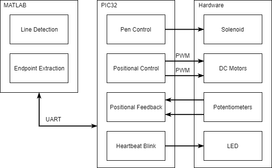
The basic logical structure of the image plotter consists of a high level MATLAB image processing section on a PC, a low level C hardware control section on the PIC32, and UART serial communication between the two. The MATLAB user interface takes an image file as input (currently only *.png files, but easily extended to other formats) and extracts the endpoints of the most prominent line segments in the image. These endpoints are sent via a USB to UART cable to the PIC32, which stores the endpoints. The microcontroller uses the mathematical relation between X and Y motor speeds and the slope of the line to decide how to recreate the line segment, then does so, actuating a solenoid to drop the dry erase pen to the whiteboard surface. It uses potentiometer readings as feedback to know when to stop the motors and lift the pen.
Originally, we planned to do image processing on the PIC32 itself, with the computer only providing the image file. This proved to be difficult, as the microcontroller has limited memory, and the space required to store an image as well as its processed data grows very quickly with image size. We found it more practical to offload the image processing to MATLAB. Since MATLAB has functions available that can very efficiently process images, and C code is more suited for controlling hardware, this approach effectively divides the two parts of our project to where they are best performed. UART serial communication makes it easy to bridge the gap between the two sections.
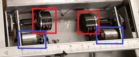
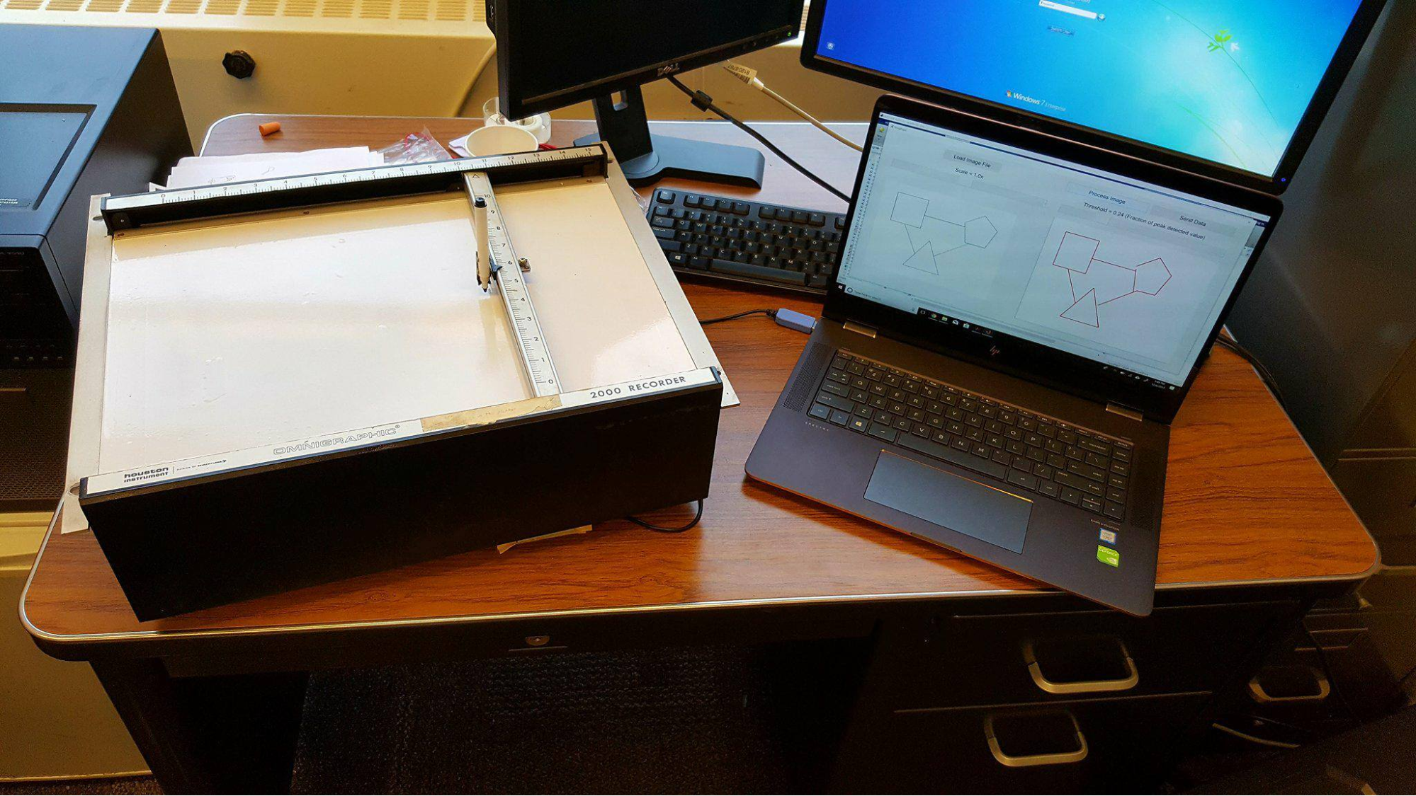
As shown in the system block diagram, the hardware is divided into four main categories: solenoid control, motor control, potentiometer feedback, and a simple LED circuit to serve as a heartbeat. The motors, solenoid and potentiometers were attached to a Houston Instrument Omnigraphic 2000 pen plotter obtained from the course instructor. The motors controlled X and Y axis motion with each shaft also attached to a potentiometer for positional feedback while the solenoid controlled the pen actuation. The components can be seen in the figure below, with potentiometers boxed in red and motors boxed in blue.
Various hardware peripherals on the PIC32 were also used. PWM was done using four Output Compare (OC) units assigned to Timer2 as the base. The onboard ADC was used to read the potentiometer inputs and general GPIO pins were used to output the heartbeat as well as the solenoid. A detailed pin-assignment table can be found below, as well as the PIC32 small development board provided.
|
Use |
Peripheral |
Pin |
|
UART |
U2RX |
RA1 |
|
U2TX |
RB10 |
|
|
X position |
AN2 |
RB0 |
|
Y position |
AN3 |
RB1 |
|
HBT_LED |
RPA0 |
RA0 |
|
X_MOT_A |
OC4 |
RB13 |
|
X_MOT_B |
OC2 |
RB11 |
|
Y_MOT_A |
OC1 |
RB15 |
|
Y_MOT_B |
OC3 |
RB14 |
|
SOLENOID |
RPB5 |
RB5 |
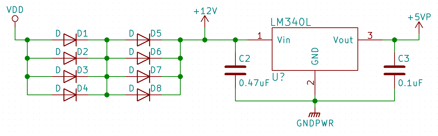
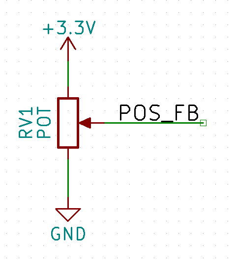
In addition, there are two planes of power that the hardware is run on, one isolated plane for the microcontroller, LED, and potentiometers, and a noisy power plane powered by an external 13.5V power supply for the motor and solenoids. The motor and solenoid power plane should be completely separate from that of the microcontroller in order to avoid large inductive voltage spikes on microcontroller pins. On the isolated plane, the only voltages are 3.3 and GND, but different voltages are needed on the unisolated side. The motors and solenoid used to move and actuate the pen run on 12V, so the 13.5V supply needed to be stepped down. This was achieved through 2 diodes in series as each has a drop of around 1.2V. However, the motors draw more than 0.5A each and the solenoid 0.5A, so we estimated a maximum continuous current draw of 3A. Each diode was rated for 1A so we put 4 in parallel in series with another 4 in parallel to make sure the diodes could handle the load. This can be seen in the schematic below.
Additionally, the H-bridges for motor control required 5V as input, so the LM340L was used to convert the nominal 12V from the diodes to 5V.
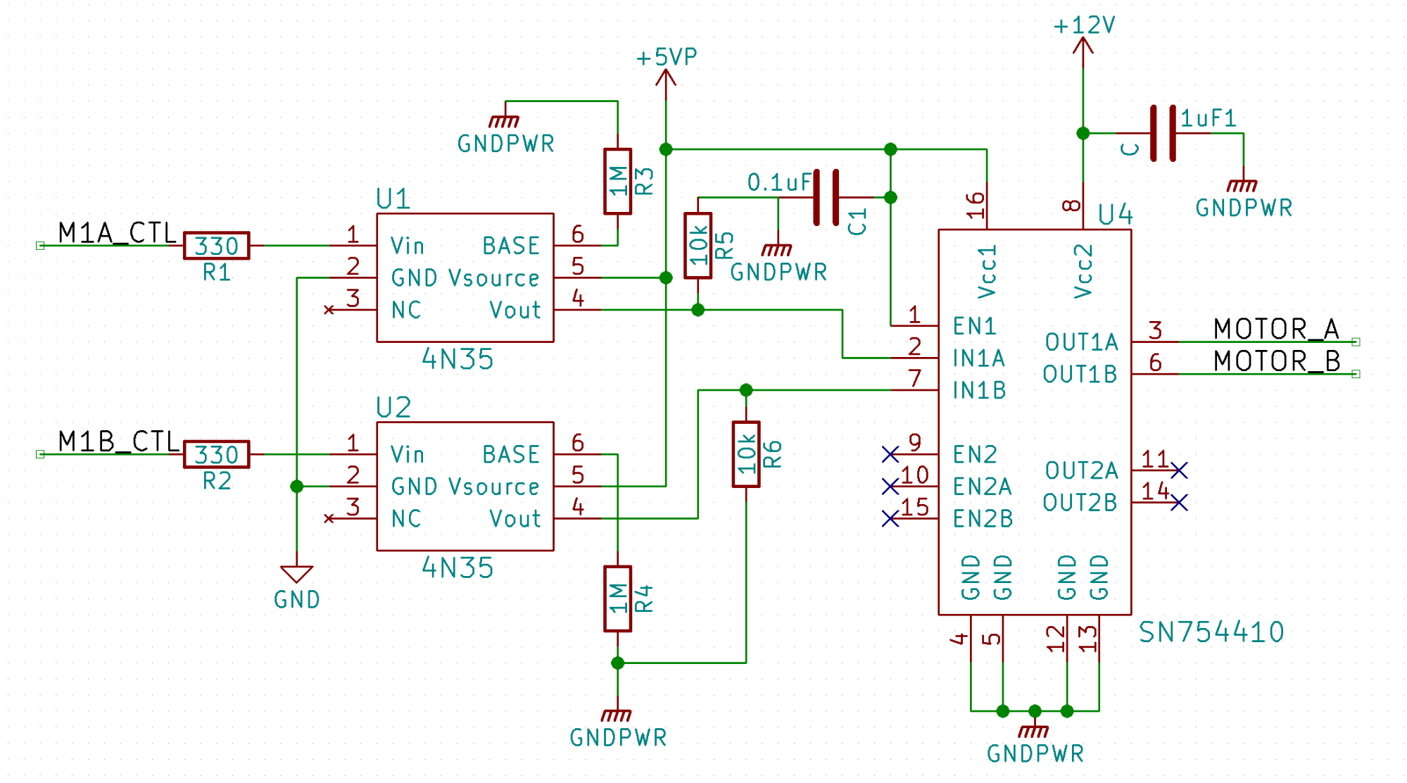
As noted above, the motors and solenoid are on a separate power plane than the microcontroller. The isolation between the two planes is achieved through the 4N35 optoisolator. PWM signals are sent from the PIC32 to the 4N35 which then outputs the unisolated 5V on the other. These signals then feed into the SN754410 quad half H-bridge chip which controls our motors. The chip has built-in flyback diodes so further protection is not required. An image of the control system can be seen below. Filter capacitors are attached at the power inputs of the SN754410 to protect against noise in the power line.
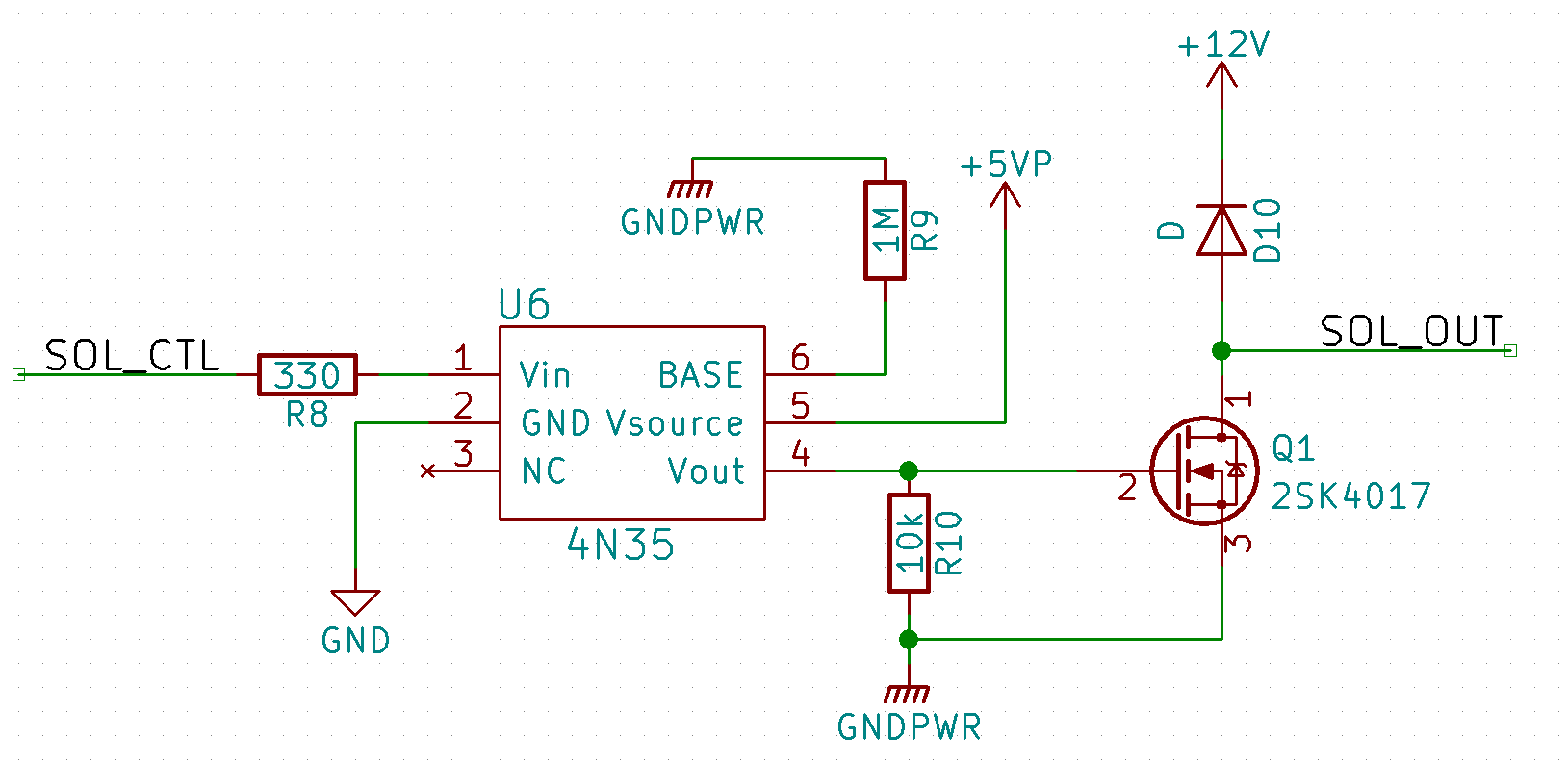
The solenoid is controlled in much the same way as the motor, but with an NFET replacing the H-bridge as only the solenoid has no notion of directionality. A flyback diode was included as well, as can be seen in the diagram below.
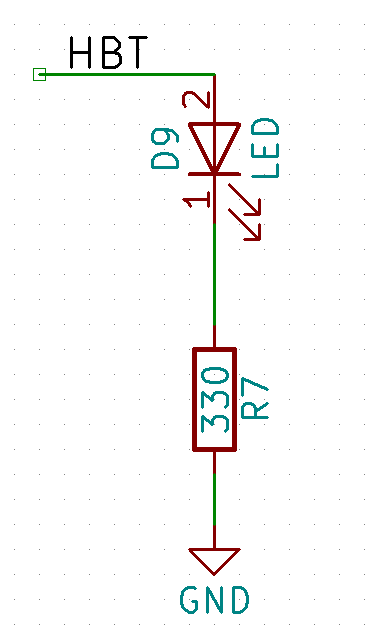
We thought it prudent to include a heartbeat LED to indicate that the PIC32 was working and threads were being scheduled with no deadlock or infinite loops. The circuit was a simple LED in series with a resistor, the schematic of which can be found in the appendix.
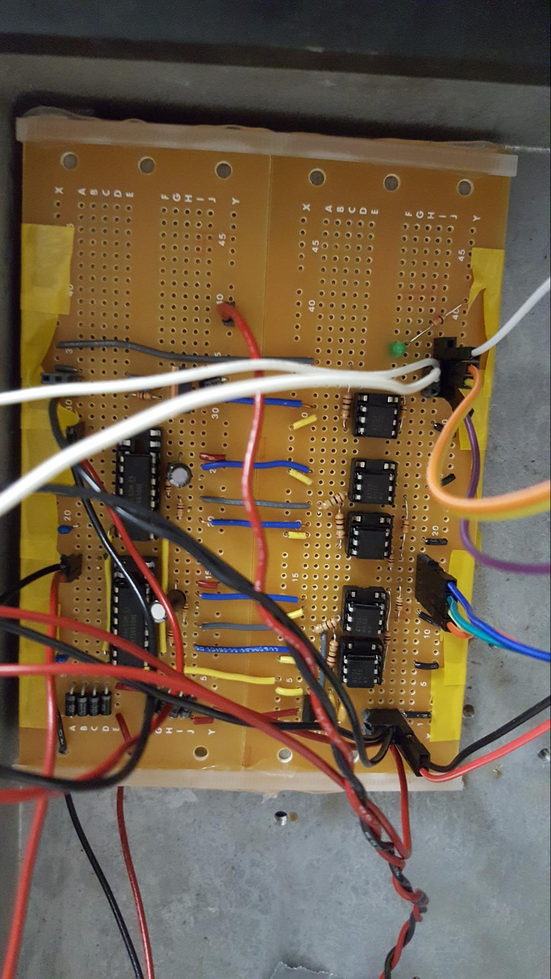
Originally, we created a prototype on a breadboard. In order to save costs, we recreated the prototype with almost the same layout on solderable perfboards.
This interface allows for choosing an image, rescaling it to fit on the plotter, processing it, and sending it over a wired UART serial connection to the PIC32.
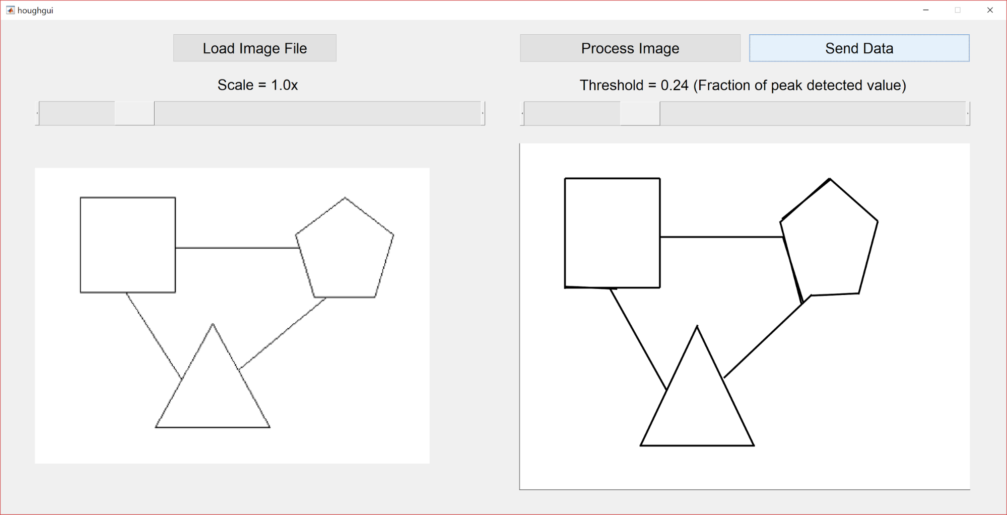
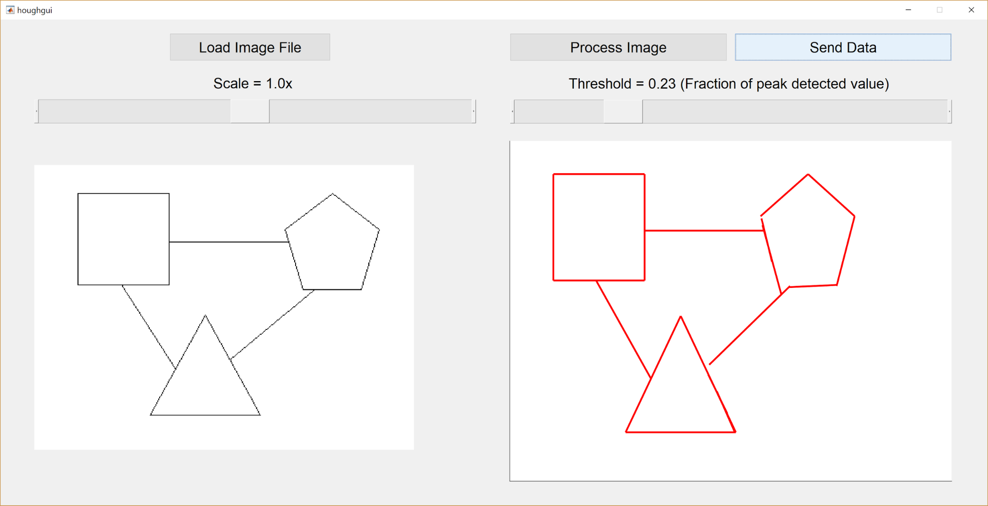
The MATLAB GUI (pictured below) allows the user to load an image file from memory, which displays on the left side of the GUI. A “Scale” slider controls the size of the image, so a 0.1 scale would result in an image one tenth the size of the original, and 1.0 would result in the original image. The image is displayed on axes allowing for a maximum 466x308 pixel image, which was determined to be the largest coordinates our motor control logic could handle based on the size of the plotter. In our coordinate scheme, we have a size scaling of about 30 pixels of image size to 1 inch on the plotter. If the image is too large to fit on the plotter after scaling, this will be evident on the displayed image, and it can be rescaled further down. Once the image is resized such that it can fit on the plotter, the actual processing can begin.
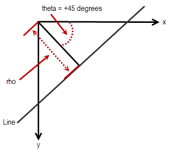
The “Process Image” button on the GUI performs our image processing on the image and prepares the line segment endpoint coordinates for transmission. It uses a Hough transform (using the MATLAB function hough) on the black and white version of the image to determine the prominent lines in the image. By default, the function looks for light lines on a dark background, but given our intended application of diagram reproduction, we take in images with dark lines on a light background and invert the colors before feeding it into the hough function. The Hough transform essentially keeps a 2D histogram of all the possible lines in the image, iterates through all the filled pixels of the image, and increments the spaces in the output matrix that represent the lines that pixel could lie on. By the end, the spaces in the matrix that have the highest values represent the most likely parameters of lines in the image. It represents lines in their polar representation, with the perpendicular distance from the origin and the angle of that perpendicular line from the x axis. See the image below for the visualization of this scheme; the y axis extends downwards by convention for graphics purposes. We used the parameters of 1 degree accuracy for the angle and 1 pixel accuracy for the distance. We found empirically that this allowed for fairly accurate image representation without detecting extra lines when the image has thicker lines. The user can utilize a slider on the GUI to change the threshold value for the built in houghpeaks function, which determines when a line becomes considered as important. The line is considered if it has at least a value of the threshold value times the max value in the output matrix. Therefore, a higher threshold will generally result in fewer lines detected, and vice versa. We also implemented a maximum number of lines as 1500 to make sure the PIC32 had enough memory to store all the coordinates.
Image from Mathworks hough documentation
The next step is to determine the endpoints of the thresholded lines. This is done using the built in houghlines function. Endpoints are inverted in the Y direction (since graphics convention is Y coordinates growing downwards instead of upwards), corrected if they stray outside of the 466x308 max size, and compensated for overshoot. Overshoot compensation is discussed in Results: Overshoot Correction.These endpoints are then converted into a format for transmission. We used 16 bit integers as the data format for our coordinates. This meant that each coordinate would be decomposed into two 8 bit characters concatenated with each other, as serial communication sends a byte at a time. Each “chunk” of transmitted data consists of 4 coordinates: the (X,Y) position of the start point and the (X,Y) position of the end point. This means the chunk is 8 characters long. Since the number of line segments is variable between different images and different thresholds, we used a chunk of the character value 0 repeated 8 times as the “stop” signal. Since the images in MATLAB are indexed from 1, this is never a valid coordinate. The processed line segments are displayed on the axes on the right side of the GUI for the user to determine whether the processing was satisfactory. If not, the threshold can be adjusted and the endpoints will be recalculated upon pressing the “Process Data” button again. Once the processed image looks good, the user can click the “Send Data” button to start the UART transmission to the PIC32.
A header file containing configuration parameters for the PIC32, provided by the course instructor, Bruce Land. The use_uart_serial definition was uncommented to enable UART use.
A header file containing macros for a PIC32 compatible Protothread implementation by the course instructor, Bruce Land. The Peripheral Pin Select call was changed to put the UART2 RX input on RA1 instead of RB11.
Our main file. All source code for PIC32 control is contained in this file.
The main function contains the setup code for the various peripherals used. This includes Timer2 and its interrupt, OC units 1-4, the ADC, and setting the GPIO pins used as digital outputs. The ADC was configured to autosample from two sources, AN2 and AN3. Finally, the protothreads are initialized and scheduled.
This ISR is responsible for the positional feedback as well as the control associated with that. Running at 1kHz, the ADC is sampled to get the current X and Y position. Then a check is performed to see if the plotter has reached its destination along the X and Y positions. If it has, a flag is set for each axis and the PWM signals to the motors are killed respectively.
It was also in the ISR that we attempted to fix the observed overshoot problem (more in the Results section), where the pen would plot around 2 inches past its desired location. First, we increased the timer frequency to 5kHz, but the overshoot remained the same, meaning the sample speed was not the issue. We theorized the overshoot was caused by motor drift. To alleviate this, we also attempted to apply a short reverse pulse, but the control for this was too complicated. We also tried to lift the pen earlier, but this would cause problems for shorter lines. In the end, we were not able to fix the overshoot within the PIC32 C program.
This function takes an integer 1 or 0 as an input and engages the solenoid when the argument is 1 and disengages if the argument is 0. This process takes some time electrically, so a wait must be implemented outside of the function.
These functions precisely set the X and Y positions of the plotter to the input argument. This is done to go to the start point of each line segment. The direction is calculated and the motors are set to run at around ⅓ power to move slowly to set the positions as precisely as possible. The done flag in the desired direction is cleared while the other is set so the system only waits on the desired axis. An external wait until the flags are set is necessary outside of these functions.
moveTo() function
This function behaves much the same way as setX() and setY() but also takes slope calculations into account. When the slope is less than 1, it becomes a linear function of the Y motor speed with the X motor speed set to max. When the slope is greater than 1, its inverse is a linear function of the X motor speed with the Y motor speed set to max. The speeds are set based on the calculated slope of the line from the current position to the desired position with speeds set accordingly. Then, based on the direction of movement, the correct PWM channels are set to the desired speeds and the movement flags are cleared. However, if the motion is close to purely horizontal or purely vertical, only the flag for the axis of major motion is cleared with the other set. This is due to the inability to draw lines whose slope or inverse slope are too close to 0 due to the movement characteristics of the DC motors. If both flags are cleared, the minor axis of motion will never be reached and the system would hang. Like the setX() and setY() functions, an external wait until the flags are set is necessary outside the function.
This thread accepts endpoints from the MATLAB interface before beginning to send commands to the motors. Since these two things happen in sequence (all endpoints are received before motors start moving), it seemed rational to include both these functionalities in a single thread. The UART portion loops until it either reaches the set maximum number of lines (set to 1500 for now to accommodate for PIC32 memory capacity) or it receives the “stop” signal of all zeros. Within that loop, it loops 4 times, receiving 2 characters during each loop, to receive the full endpoints of the segment as 8 characters. It shifts the first character left by 8 bits and ORs it with the second character in order to concatenate them, recovering the 16 bit integer coordinate that was sent. Each coordinate Xstart, Ystart, Xstop, and Ystop is placed into separate arrays, so that all values corresponding to a certain segment have the same index within their array. The array is populated by all the endpoints that were sent.
Then, for each line segment received, the thread will set the current position to the start point with the setX() and setY() functions. Each is followed by a call to PT_YIELD_UNTIL with xflag and yflag as the condition. In addition, a yield of 0.25 seconds is used to make sure the system has completely come to a stop. After setting the start point, penEngage(1) is called to engage the pen followed by a pause, followed by moveTo(endpoints) with the same yield conditions as setX() and setY(). Finally, the penEngage(0) is called to disengage the pen and the loop repeats. After all points have been drawn, the entire thread repeats and waits for more coordinates for a new image over UART.
This thread simply blinks and LED on and off every second to indicate that no deadlock or infinite loop has occurred.
Our end result was that our plotter faithfully recreated images as long as they contained only straight lines. However, due to both hardware and software limitations, there are some constraints on the angles of lines the plotter can reproduce.
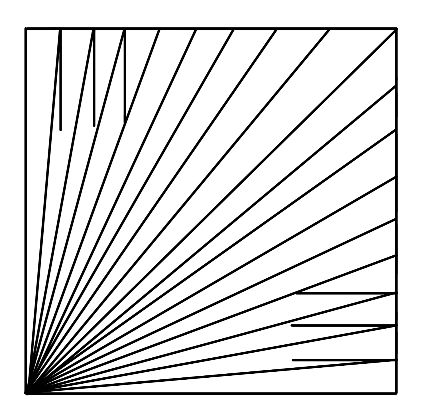
The hardware angle limitation comes from the fact that too low of a PWM value does not provide enough power to move the motors, and even slightly above that limit, the rail and pulley system used to move the assembly provide enough resistance that motion is not smooth, which would not create a straight line. This effectively limits the angles of lines we can draw to horizontal, vertical, and anything between around 5 and 85 degrees in all quadrants to +2o accuracy. The test image shown below was used for this angle accuracy, with lines at increments of 5o.
While it is not truly continuous due to the discretized nature of our PWM duty cycle (out of 40000), the granularity is far finer than what our application calls for (1 degree: more on this design choice in the Program Design section above).
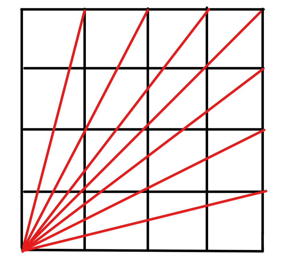
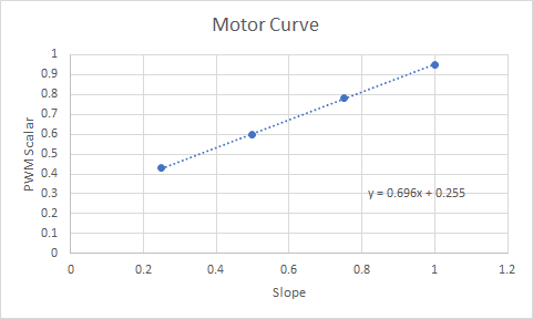
Through testing and calibration, we found that the slope of lines we wanted to reproduce was linear with the equation PWM Scalar = 0.696 * slope + 0.255 where PWM Speed = 40000 * PWM Scalar. This was done by making the plotter draw a square split into a 4 x 4 grid and attempt to draw lines from the bottom left corner to each intersection along the outer edge, as shown below, by hard coding PWM duty cycle values.
For slopes less than 1, we recorded the slope as well as the PWM scalar for Y speed that yielded that slope with X speed held constant at the maximum value. We plotted the data and calculated a curve of best fit using Microsoft Excel. The plot and fit line is shown below.
Through further testing and experimentation, the same equation works for lines whose inverse slope is less than 1 by applying the scalar to the X speed while holding Y speed at max.
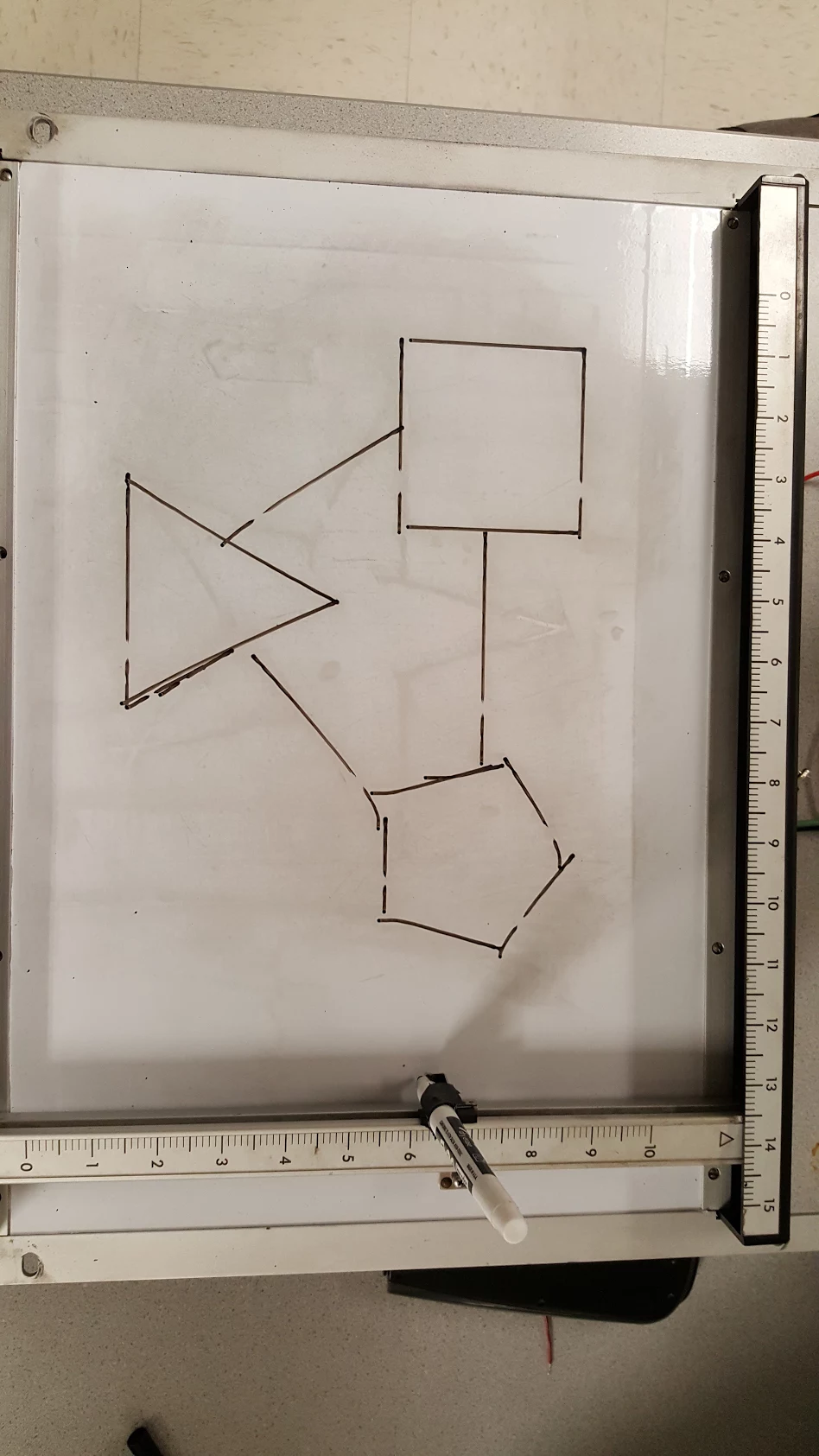
One issue with accuracy is the problem of overshoot. Our lines tend to extend about 1.5 inches further than they should. We originally thought this might be a product of sample rate with the ISR, but increasing the frequency did not change the overshoot. Also, on lines with angles between 45 degrees and flat, the overshoots curve with the concavity facing the axis with the faster speed. This led us to believe the overshoot was caused by motor drift, or slow braking. When we command the motors to stop, both terminals are grounded, which should drain the motors and brake, but it occurs too slowly. We attempted to apply inverse pulses and to lift the pen earlier, but both attempts were unsuccessful. However, the image was still recognizable and after erasing the overshoot, very accurate. An example of an image with overshoot and with overshoot removed is compared here.
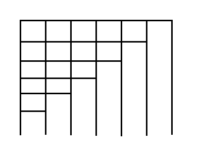
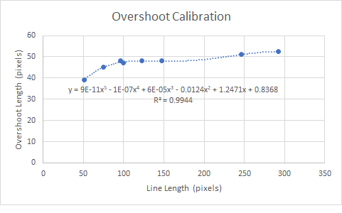
In order to correct for overshoot, we needed to do some more data collection. We found that the amount of overshoot distance was not constant but instead depended on original line length, with longer lines being drawn with longer overshoots. We created a test image with several horizontal lines of varying length and vertical lines intersecting them at their endpoints to determine the desired endpoint of the line. We sent this image to the plotter at full scale and half scale, measured the original line length as well as the overshoot length, and fit a curve to the data. The test image, plot, and best fit curve are shown below.
The fifth order equation shown is used in the MATLAB processing code to subtract the calculated distance off of a line before sending the adjusted coordinates. Following this, the drawn line plus its overshoot should be approximately equivalent to the original desired line. The same drawn image as before is displayed again below, but with overshoot compensation implemented.
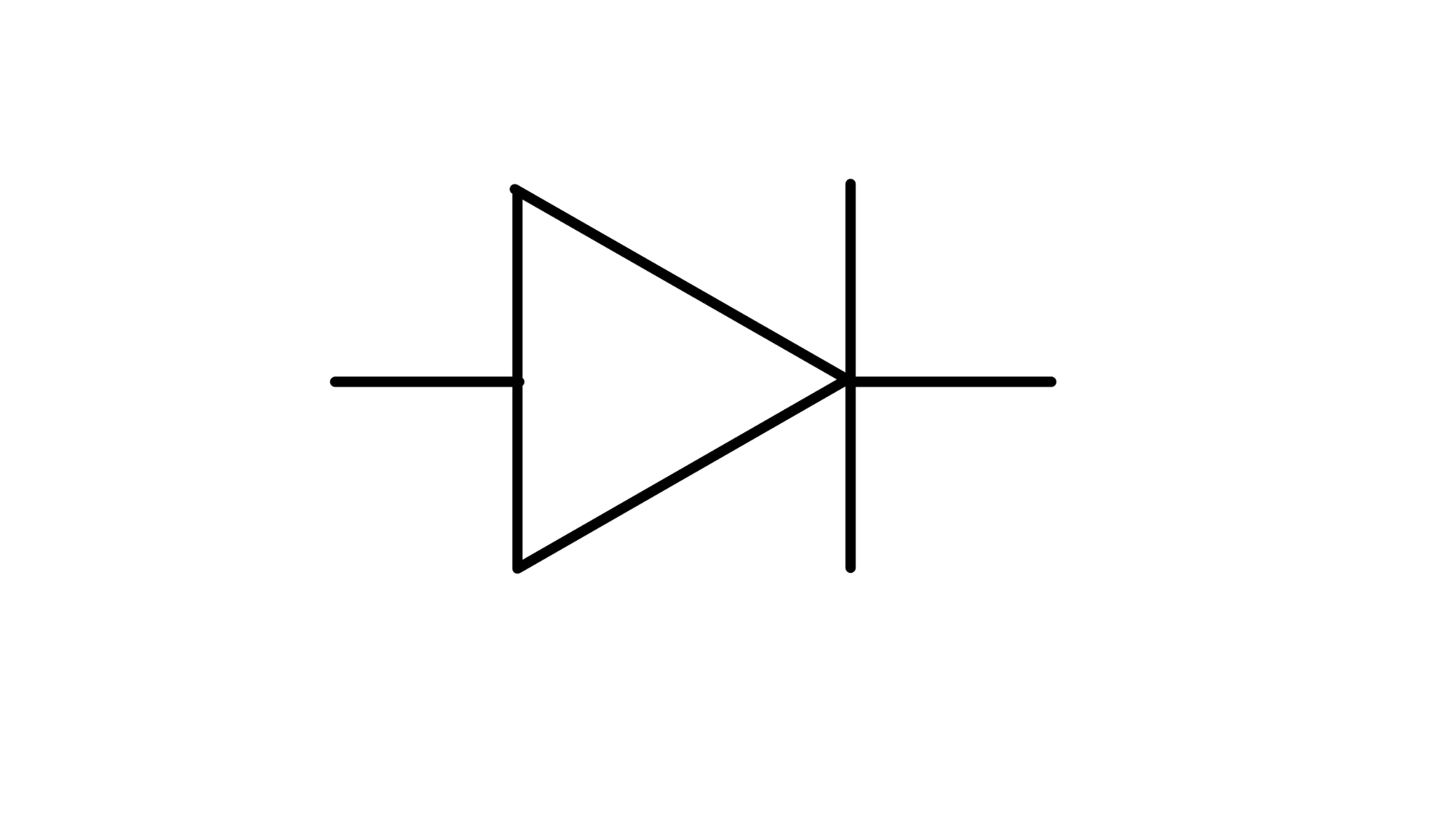
As for speed of performance, an approximately 4”x6” image of a diode containing 6 lines (shown below) took 18 seconds to complete. The test image from above containing the square, triangle, and pentagon at a total size of about 9”x11” took 52 seconds to complete. This includes time to readjust and time to draw lines. Readjusting pen speed is approximately 3 inches per second and drawing speed is approximately 10 inches per second.
Finally, the GUI proved usable and intuitive. It accurately represented how an image would appear on the plotter whiteboard in terms of location and size. It allowed for dynamic rescaling and reprocessing of the image so that it could be determined to be a good image before sending the information to the PIC32.
Performance versus Expectation
The image plotter met our set specification of being able to recreate an image consisting of line segments on our whiteboard. It does have some difficulty with lines of extreme shallow or steep slopes since there is a lower limit on motor speed, as described in Program Design: moveTo() function. The finished prototype should still be sufficient to recreate any basic line-dominated image, such as diagrams - our initial focus.
The main problem we experienced was the overshoot problem described in Results: Overshoot Correction. Even with our curve fitting, there are still some minor overshoots and undershoots, but compared to having no overshoot correction, it was leagues improved. The motor drift and slight irregularities in resistance of movement along the rails were not ideal, but by using high movement speeds and software correction, they were mitigated quite well. Overall, the plotter met our expectations.
Our project was written in C, using the C99 specifications and also utilized USB for serial UART communications. UART communication with 8 data bits and 1 stop bit was used. None of these standards were implemented by us, only used. There should be no legal issues, as reverse engineering, as we did with the Omnigraphic 2000, is legal, and any patents on it are old enough to have expired.
The plotter itself was not our work, simply the control circuitry, code, and application. As mentioned in the Hardware Design section, the Houston Instrument Omnigraphic 2000 was gutted and the original movement mechanisms, potentiometers, motors, and solenoid were used. However, as the device was released in the 1980s, any sort of patent on it should be expired.
The MATLAB user interface was constructed using GUIDE, a MATLAB app for creating custom graphical user interfaces. The image processing algorithm was designed with reference to the Mathworks documentation for hough and houghlines.
We may pursue publication in a hobbyist magazine in the future.
As mentioned in the introduction, part of the motivation of this project is to reduce waste. It is just as simple to print a diagram as it is to redraw it using our image plotter. However, it is a waste of paper to print out diagrams or images for scratch work. It is much more environmentally friendly to use a whiteboard as we have, so nothing is thrown away and the surface can simply be reused for the next image. It could potentially reduce waste in many students’ situations of needing to draw or mark on diagrams.
Safety was held as first priority during the execution of this project. Because of the high current requirements of the motors and solenoid, there are about 3 amps of current at 12 volts flowing through our circuits during operation. This kind of power can be dangerous, so precautions need to be taken. We put together a soldered perfboard with all the control circuitry to ensure that long jumper wires were not scattered throughout the project. The whole conducting side of the board was insulated using electrical tape, and then the electrical boards were secured to the underside of the plotter to keep any users out of danger.
The group approves this report for inclusion on the course website.
The group approves the video for inclusion on the course YouTube channel.
Positional Feedback and Heartbeat
Motor Control
Power
Solenoid Control
Click part for datasheet, click acquisition for vendor site.
|
Part |
Acquisition |
Qty |
Unit Price |
Notes |
|
MicroStickII |
Lab |
1 |
$1.00 |
Programmer |
|
Small Board |
Lab |
1 |
$4.00 |
|
|
Solder Board (6”) |
Lab |
2 |
$2.50 |
|
|
13.5V Supply |
Lab |
1 |
$5.00 |
For motors/solenoid |
|
5V Supply |
Lab |
1 |
$5.00 |
For PIC32 |
|
PIC32 |
Lab |
1 |
$5.00 |
|
|
Jumper Wires |
Lab |
10 |
$0.10 |
|
|
Header/Sockets |
Lab |
32 |
$0.05 |
|
|
Various Passives |
Lab |
- |
$0.00 |
Resistors, Capacitors, Diodes |
|
Lab |
5 |
$0.00 |
|
|
|
Lab |
1 |
$0.00 |
|
|
|
Plotter |
Salvage |
1 |
$0.00 |
Given by Bruce Land |
|
2 |
$2.52 |
|
||
|
USB to TTL Cable |
1 |
$9.95 |
|
|
|
Total Cost |
$42.59 |
|||
A fully commented listing of our code can be downloaded below.
Patrick worked on gutting and figuring out how to interface with the original plotter, circuit design and motor control code on the PIC32.
Rohan worked on UART communication, MATLAB image processing and GUI design, and soldering the final perfboard based on Patrick’s prototype.
All hardware testing and debugging was done as a pair.