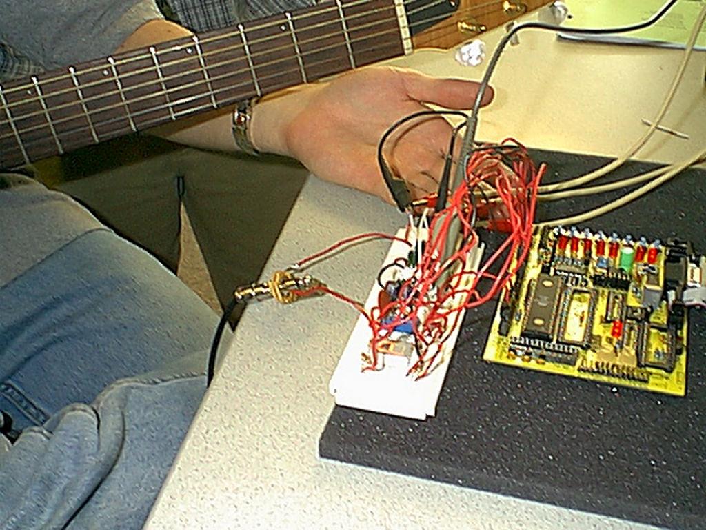
Introduction

The goal of this project is to design an algorithm for a real-time digital guitar tuner and implement it using an Atmel AT90S8535 microcontroller. Each of the six strings of a guitar has a unique fundamental frequency, and our goal is to measure this frequency and compare it to the correct frequency. This project combines digital filter design, analog amplifier design, and several data analysis techniques.

High level design

The microcontroller accepts push button inputs which allow the user to select which guitar string is being tuned. It then samples the input waveform at 3000 Hz using the 8535's on-board ADC. Each time a waveform sample is obtained, the following FIR (finite impulse response) filter algorithm is performed:

where P = 21, x_n are the most recent 21 samples and c_i are predetermined filter coefficients which are loaded from a lookup table for each string. This filter set to be a bandpass filter centered at the fundamental frequency of the selected guitar string, and it is used to remove unwanted harmonics and other noise from the sampled waveform. Note that we are limited to a 20-tap filter (P = 21) because all operations must be completed within one sample period (.333 mS) in order for the tuner to be true real-time. Generally speaking, the larger P is, the better the filter is.

After each filter output has been calculated, it is examined to see if it is a rising-edge zero-crossing. The number of sample periods between rising-edge zero-crossings is recorded and averaged, and the result is the fundamental period of the guitar tone. This fundamental period is compared to a series of threshold levels, and a single LED is illuminated to indicate the sharpness or flatness of the tone. The threshold levels (from LED0 - LED7 on the evaluation board) are fundamental +15%, +10%, +4%, +1%, -1%, -4%, -10%, and -15%. If the measured period falls within +1% and -1%, the two middle LEDs are illuminated (LED3 and LED4).

MATLAB Simulation

Extensive MATLAB work was done before the first line of assembly code was written in order to determine whether or not the algorithm could be implemented on the 8535. There are many limitations of the 8535 that we had to consider. In order to perform all of the necessary calculations within one sample period, the multiply routines need to be as fast as possible.

Our original plan was to implement a 2-pole Butterworth IIR (infinite impulse response) filter, since it requires few multiply operations and achieves a very nice frequency response. However, this algorithm is very sensitive to the filter coefficients, and it is also very sensitive to it's own output since it is recursive. Using MATLAB, we created a model for how the 8535 would represent the filter coefficients and output values, and we tried to make it work. The results indicated that even using 16-bit resolution for the coefficients and outputs, the filter was extremely unstable at times and unresponsive at others. As one example, rounding the coefficients to the nearest representable 16-bit number could cause the filter frequency response to vary radically, deeming it unstable. As another example, the filter outputs were represented in 32 bits, but needed to be reduced to 16-bits for the next filter iteration. The process of reducing 32-bit resolution to 16-bit resolution often eliminated all significant digits, and the filter would never "start". Instability and unresponsiveness are common problem with IIR filters.

Our second plan was to implement a 21-tap FIR filter, which is more cooperative than an IIR since it is non-recursive. That is, the present filter output does not depend on any previous filter outputs. However, an FIR filter requires many more multiply operations to achieve the same frequency response as an IIR filter. An 8-bit by 8-bit multiply routine requires only 34 clock cycles to complete, whereas a 16-bit by 16-bit multiply requires105 clock cycles. Therefore, in order to implement a filter with a reasonably large P, we need to use the 8-bit multiply routine. With only 8 bits of resolution for our filter coefficients, we needed to evaluate the sensitivity of our FIR algorithm. Again, we created a MATLAB model for how the 8535 would represent the filter coefficients, and used it to determine we could implement a sufficient filter. The results indicated that we could.

For comparison purposes, the following three figures show frequency responses for a 2nd order Butterworth filter, a 20-tap FIR filter (the one we used), and a 100-tap FIR filter. All filters have a cutoff frequency of 247 Hz, and a bandwidth of 70 Hz. This is the filter shape required for the second guitar string (B). As you can see, both the 2nd order Butterworth and the 100-tap FIR perform well. However, for reasons explained above we had to settle for the 20-tap FIR. Although the 20-tap FIR does not look as good as the other two, it gets the job done. The red lines in the figures show the designed passband.

Software

 The nature of a real-time DSP system requires that we complete all our computations between ADC samples. At a sampling rate of 3000 Hz, we are left with 333 microseconds to complete our task. At 4MHz, this translates into 1333 clock cycles, which turns out to be not enough (21 multiplies sucks up a lot of clock cycles). To solve this problem, we replaced the 4MHz oscillator with an 8MHz one, providing a new total of 2666 cycles to work with.

By far, the most complex portion of our code was that which implemented the FIR filter. The first step was to place the coefficients, 21 8-bit values per string, in SRAM. Although the EEPROM would be a viable alternative, we feared that the slow access times could possibly hinder our performance. Therefore, immediately after the reset and register setup, we load our coefficients into contiguous locations in SRAM. The coefficients could then be accessed by setting a pointer (X, Y, or Z) to the beginning of a coefficient memory block.

The mathematically intensive nature of the FIR calculation required that we utilize some tricks to make it work within the allotted clock cycles. Because we knew that all of the values returned by the ADC would be positive integers (between 0 and 255), we were able to use unsigned multiplication (much faster than signed) in our algorithm. Although the filter coefficients did vary in sign, we were able to circumvent this problem by storing the signs of the members of each coefficient set in memory along with the unsigned coefficients themselves. Thus, we performed unsigned multiplies and then added or subtracted our result from our running total based upon the sign of the coefficient.

Once the filter produces a result (about once every 333 microseconds) we have to process it and use it to determine the frequency of our input. To accomplish this, we count the rising-edge zero-crossings of our output. This is implemented by watching the sign bit (MSB) of our result; when it goes from 1 (negative) to 0 (positive), we know a positive rising edge has occurred. By counting the number of sample periods between these rising edges, we can measure the period of the waveform, and consequently the fundamental frequency of our input. This algorithm assumes that the output of the filter is sine waves with a frequency equal to that of the fundamental of the string we are playing. Although this assumption is mostly true, there are cases where distortions in the output caused by ineffectively filtered harmonics can cause spurious zero-crossings at frequencies other than the fundamental. To deal with this, we made our zero-crossing detection "smart" by ignoring those detected periods which were not within an appropriate range of the fundamental (25% plus or minus).

Finally, we are ready to display our output on the LED's. We proceed by comparing our period value with a series of thresholds contained in .EQU statements. We light our LED's accordingly: the higher order lights indicating a sharp note, the lower order lights indicating a flat note, and the two center lights indicating a correct fundamental frequency.

 Click here to see part 1 of the source code.
 Click here to see part 2 of the source code.

Debug Software

In order to determine if our MATLAB model would actually work in the 8535, we had to see what our inputs looked like once they were sampled by the ADC. Displaying the ADC values to the LED's is of no use, as a new one would appear every 333 microseconds, making it impossible to discern the values. We decided the solution was to use the UART; however, attempting to output the values to the UART in real time turned out to be impossible. Even at 38400 baud, the allotted time between samples only gives us time to transmit 12 bits! That's just over one character; not enough for our purposes. The solution was to forgo the real-time implementation for one that reads in 300 samples and then outputs them. Our ADC debug code stores 300 8-bit ADC samples in successive SRAM locations and then the UART outputs the stored values at 9600 baud.

 Click here to see debug source code.

Hardware

A DC-coupled amplifier with a gain of 470 was designed to amplify the signal from the guitar pickup to levels suitable for the 8535's ADC. The guitar produces a maximum voltage approximately 5 mV-pk, so the amplifier boosts that to 2.35 V-pk. The amplifier also applies a 2.5V DC offset to the output, and the result is an AC signal that ranges from approximately 0.15V to 4.85V. This is well suited for the 8535 ADC's input range of 0V - 5V. This amplifier gain works well, although if the guitar string is plucked too hard the output will become too large and will be clipped by to op-amp. The following is a schematic of the amplifier:

A second circuit, a fourth-order Bessel lowpass filter, was built in anticipation of aliasing problems with the A/D converter. This filter was designed with a cutoff frequency fc = 375 Hz (-3 dB @ 375 Hz), and attenuates at -24 dB per octave beyond fc. Any aliasing problems would result from frequencies above our Nyquist frequency of 1500 Hz, and this filter does a very good job of eliminating those. As it turns out, no aliasing problems occurred so the filter was not needed. For reference, the following are the schematic and frequency response of the filter that was designed:

Results

There are two levels of results that can be reported. The first is overall accuracy of the tuner. We tuned a guitar using our tuner and then measured the fundamental frequency using an oscilloscope. The frequencies we measured were all very close to those that we designed for. Since the digital scope introduces a bit of time quantization error, it was not possible to take exact measurements. A second test we performed to analyze our results was to measure our tuned guitar with a commercially available guitar tuner made by Korg (retail price ~$50). This tuner is extremely sensitive to frequency changes, and is therefore a better metric to use than the scope. What we found was that in all cases, our guitar was perfectly in tune according to the Korg instrument. (Okay, okay... it wasn't that accurate the first time, but we were able to tweak it). One slight problem we noticed was that for a few strings, there is too much "play" in the tuner. That is, the range of frequencies for which the tuner tells us we're in tune is a bit too wide. This also can be tweaked.

A second level of results that we examined was the filter response. Since implementation of the filter algorithm was such a large part of our project, we felt it necessary to do this. Using the debug version of our program described above, we were able to record the sampled waveform and filter output as calculated by the 8535. The two waveforms were plotted together using MATLAB, and the results for two strings are shown below. Notice in each case that the sampled waveforms (blue) are distorted the overtones (harmonics) of the guitar sound, and are also clipped by the ADC. In both cases, the filter output is much cleaner. Since we're only able to implement a 20-tap filter, the output is not a perfect sine. However, the harmonics are drastically reduced and therefore it is easy to calculate the fundamental frequency.

 
 

What to do differently next time

 This type of filter algorithm is not very well suited for an 8 bit RISC architecture such as the 8353. In order to design a good filter it is necessary to perform multiplication operations with great resolution (IIR algorithm), or multiplication operations with less resolution but with great speed (FIR algorithm). The 8535 is capable of neither. A single signed 16-bit multiplication requires 250 clock cycles, making an IIR algorithm difficult. A single unsigned 8-bit multiplication requires 34 clock cycles, limiting the number of taps that can be implemented for an FIR filter. The right way to do a project like this is to use a dedicated DSP architecture, which can perform complex operations such as 16-bit signed multiplication at the hardware level in one clock cycle.

Useful links...

Time domain filtering techniques for digital audio - a good overview of digital filters with some filter design tools.

Interactive Digital Filter Design - a better tool for filter design.

Guitar Fundamental Frequency - a complete table of fundamental frequencies for guitar tones.

Preamp Construction Articles - a good source of info for preamp design.

Basic Circuit Blocks - Active Filters - cookbook-style approach to analog filter design.