EE 476 Final Project
Autonomous Vehicle
Contrast Following Rover
By Reid Gurnee and James Barabas
INTRODUCTION
As technology develops, computers are making people's lives progressively easier and safer. Someday they will be able to drive automobiles, resulting in reduced deaths and accidents. We decided to make a prototype of a self controlled car. We started with a Hot Shot II radio control car and stripped out the radio receiver. Then we gained complete control over the drive and steering servos, allowing complete control of the car via the Atmel AVR8515 micro-controller.
In order to choose a non-predetermined path, we set up an array of sensors that could detect a line against a luminance contrasting surface (ie: black line on white background). The micro-controller then sensed the position of the line relative to the car and steered accordingly. To maintain constant speed, a sixth light sensor detects wheel rotation. The PWM signal to the motor is adjusted to maintain the desired speed through a digital feedback algorithm, obtaining data from the wheel.
When the car looses the line, or gets to the end of the track, it automatically stops and enters a data upload state. The speed and steering data, recorded at 10 samples/second, can be uploaded to a computer and the car's path can be reconstructed in MATLAB.
Features:
HARDWARE
Detector circuit for one detector
Detecting the Line:
To detect the line we built an array of five infrared LED’s and sensors. Each LED illuminates the floor, and the sensors detect the light reflectance. The circuit above takes the output of the detectors and turns it into a clear 0V or 5V digital output. An output high indicates a black line below a sensor, and an output low indicates white (higher reflectance surface).
The phototransistor Q1 is connected to a virtual ground through R2. U1 measure the voltage across R3 and invert amplifies it by a factor of 50. From our measurements, the voltage change across R2 from a dark line to the tile varies from .02V to .3V. After the gain stage, this difference is 1V to 15V. To get a digital output this signal is fed into an open loop gain op-amp, U2, with a reference voltage for its other input. This results in a distinct digital output of ±Vrail. LED D2 gives a visual indication of the sensor state, while also acting as a rectifier to prevent the output from dropping below 0V. Zener diode D3 breaks down in output high, clamping the output to 5.1V, resulting in a 0V to 5V digital output independent of the power supply to the op-amps. This allowed us to test using a ±15V lab supply (built in EE 114) to save the cost of expensive 9V batteries. The final 10K resistor, R6, offers current protection against any unforeseen errors.
Because U1 is inverting, the circuit requires a dual polarity power supply. This is achieved with two 9V batteries. The current draw from the batteries is fairly high because they have to drive the board, six infrared LED’s, and six indicator LED’s. To keep power dissipation as low as possible R5 is 10K, resulting in a dim indicator LED but not sacrificing performance. The ideal values for R1 and R2, and the gain of U1 were found through experimentation. We didn't power the infrared LED's on the 8.4V car battery pack because the PWM motor controller resulting in significant switching voltage noise on the battery. This would effect the line sensor readings. We tried powering the micro-controller board on the car battery pack because it has a good, noise resistant power supply, but the motor current draw was too great and the board reset during high acceleration.
We ultimately powered the micro-controller board from the top 9V battery, V2. Because the on-board power supply uses a full-wave diode bridge the board ground is 0.6V above the battery ground. We found it necessary to clamp the board ground to the true ground of the system to eliminate the 0.6V difference, otherwise the servo's didn't work correctly.
The reference voltage allows us to set the threshold where the sensors change from detecting black to detecting white. Because of the high gain and threshold voltages, the sensors were able to detect very small differences in reflectance and output them as digital results. For example, they could differentiate black tape against dark wood. Using only one reference voltage, we experienced minor consistency problems on the five sensors. These were solved by manually selecting gain resistors for U1 to obtain consistent results.
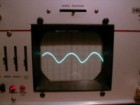
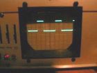
The sensor array is shielded from outside light with a black skirt. Light produced by fluorescent bulbs oscillates at 120 cycles per second. The scope output on the left shows this oscillation being measured by one of the phototransistors. Without light isolation, this oscillation could cause a PWM waveform at the output of U2 because a reference voltage is being compared to a sine-like wave. This effect is depicted in the scope output on the right. The high gain of U1 also helps reduce this PWM effect because it ensures quick transitions.
|
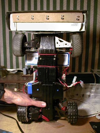
Speed detection We used a similar sensor scheme to detect the car’s speed. The inside of the rear right wheel shown above is half white and half black. An LED-sensor pair is mounted facing the wheel. This sensor detects the position of the wheel. By monitoring this sensor over time, we can determine the period of rotation of the car's wheels. The circuit is the same used for line detection, except it has it’s own Vref. | 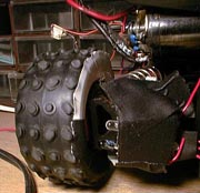 |
SOFTWARE
AVR 8515
For the control system of the car, we chose the Atmel AVR 8535 micro-controller. Running at 4Mhz, this micro-controller provides us with four 8 pin ports of I/O pins, two timers, a UART, and 512 bytes of sram.
The port pins on the MCU are connected as follows:
PORTA: Connected to 8 status LEDS on development board
PORTB: Pin 0: Connected to control line on steering servo, pin 1: connected to motor controller control line
PORTC: Connected to 8 pushbuttons on development board
PORTD: Pins 0,1: Connected to serial port, pin 2: wheel sensor, pins 3-8: line sensor
Servo Control
We found specs for servo control of the web. Depicted below is the timing diagram. The servo takes a pulse between 1ms and 2ms followed by a 18 to 25ms pause before the next pulse. The pulse width determines the servo position. TIMER1 is ideal for controlling two servos. We found that we needed a 20ms or greater period for the servos to operate correctly. Using TIMER1 with a prescale of 1 only results in a 16ms period, so we had to set the prescaler to 8. The timer is preloaded to 2^16-10000, and both servo controller pins (speed and steering) are set high. When compareA interrupts the speed control pin is pulled low, and when compareB interrupts the steering control pin is pulled low. When the timer overflows it is re-initialized to 2^16-10000 and the pins are pulled high. This results in independent control of both servos using only one timer and interrupts. At any point in our program, we can set the servo position by feeding timer 1 compare match values into four intermediate registers. Next time the timer 1 interrupt is executed, it loads these intermediates into the four timer 1 compare match registers to set servo position.
Steering
The steering position is a direct function of the sensor readout. The table below lists the steering positions and the corresponding sensor readings. The sensor array is samples at 100 times per second, resulting in almost no delay time to send the servo the appropriate reading. In the case of a faulty reading the steering stays on it's last value.
|
Steering Position |
Sensor Reading |
|
Servo Left Max |
10000 |
|
Servo Left3 |
11000 |
|
Servo Left2 |
01000 |
|
Servo Left1 |
01100 |
|
Servo Center |
00100 |
|
Servo Right1 |
00110 |
|
Servo Right2 |
00010 |
|
Servo Right3 |
00011 |
|
Servo Right Max |
00001 |
We attempted more complicated steering algorithms. Our first one samples at a constant rate and kept a steering state variable. It added or subtracted from the variable depending on the sensor reading. If the sensor reading was at center, it made no change, regardless of the position of the wheels. As the sensor reading moved towards the extremes, the steering changed by a larger amount in the direction opposite the deviation. This technique did not work as well as the simpler one we implemented.
Getting the steering to function reliably also involved optimizing constants corresponding to steering positions. We needed to make sure that when we entered a curve of a certain radius, the steering adjusted to close to that radius. When steering is configured in this way, the car does not oscillate as much between steering positions when it is on a curve. Currently, the steering positions are separated by a constant servo angle. The maximum steering positions were carefully selected to correspond to the physical steering limits of the car.
In order to get as much information as possible, the width of the line needs to be just larger than the spacing between two of our sensors (about 2"). The car can follow narrower lines, but it can steer more precisely if it is able to detect the line with two sensors at once. If the line is thinner than the spacing between two sensors, the steering can only switch to every other entry in the above lookup table (the entries with only one 1) .
When the sensor reads all 0's, we start a countdown timer. If this reading remains for .5sec, the car applies the brakes (shorting the terminals of the motor), and prepares to upload it's recorded data.
Speed Control
This car was originally a high end race car. It has competed, and won, many professional races. This basically means one thing: It's very fast. Its top speed is around 35 mph. Since our ideal detection speed is in the range of 5 to 7 mph, it was necessary to implement a feedback control system to monitor and adjust its speed on the track.
As described and depicted above, the inside of the wheel is half black, half white. Every 10ms, increments a wheel period counter the car looks at the wheel sensor. If the sensor has moved from white to black, the counter is stopped, saved, and reset. When this occurs, the program looks up the period in a table and determines the car's speed. If the reading is lover than some threshold, it is assumed that there was some bounce in the sensor transition, and the reading is discarded. Once the speed has been determined, the program compares it to the desired speed. If the car's velocity is significantly different form the desired rate, the code adjusts the motor torque accordingly. Additionally, when the sensor has not changed state in .75 sec, a speedup is invoked. Using this speedup, the car starts applying no power to the motor, and increases this power until it reaches its desired speed.
Currently, the speed feedback is a little coarse. The feedback system often overcompensates for changes in speed (particularly by panicking when it starts going too fast, coming to a complete stop). To compensate, we included a minimum time between speed changes of .5 sec. This seems to work well, but the vehicle will still occasionally slow down too much, and stop.
Data
The car stores every tenth sensor reading into sram (10/sec). When the end of ram is reached, the car continues to run, but stops trying to save it's sensor readings. After the car has reached the end of the line, or the halt button has been pressed, it sends all of the recorded data though the serial port. The MCU then waits for a g character on the serial port, and upon receipt, sends the data again. The data is stored and sent as follows: The high byte contains the steering position. A 2 indicates full left and a 10 indicates full right. A zero indicates an invalid reading, indicating that the previous steering position is still valid. The low byte of the stored data contains the car's speed on the last table lookup. A zero indicates the car is stopped, and a 5 indicates about 5 MPH.
To import this data, we wrote a C program. This program sends a 'g' to the MCU, and records the incoming stream. It separates the incoming data bytes into space separated digits in Matlab file import format.
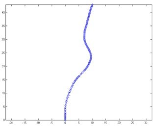
To plot this data, we wrote a short Matlab fragment. Below is a sample output.
Results
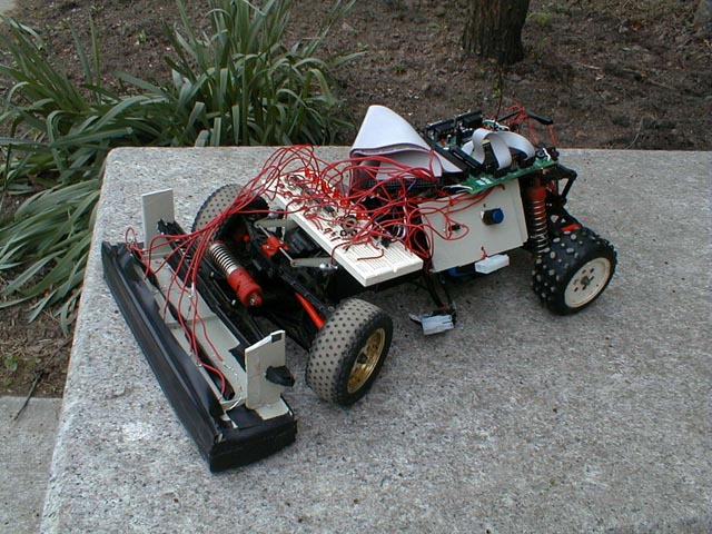
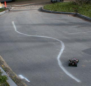
Overall, the car far outperformed our expectations. It could easily follow a black tape line on a tile floor at moderate speeds. It could also perform in non-ideal conditions. Shown above is a white line spray painted on black pavement. The line varies in width and contrast, and the background pavement is not a consistent black but a light non-uniform light gray. The robust detection circuit was also able to sense and follow this line.
The speed feedback control fell short of our expectations. We had trouble fine tuning it to obtain a consistent speed. The car would often come to a stop in the middle of the track then resume again after it detected it had stopped. The speed of the car can be easily seen from the MATLAB plot above. The data is taken at a sample rate of 10 samples/sec. The car stopped or slowed down where the data is bunched together.
If we could do it again
Throughout the design process we continually redesigned our hardware and software to optimize the car. For example, the sensor detection circuit has gone through at least four revisions. Because we continually redesigned the project, we came out with a final product that needs few changes. Our biggest problems were with the speed feedback control. If we could redo that we would put more color changes on the inside of the wheel so we know more frequently how fast the car is going. If we had more time, we also would have soldiered the circuit. Though the circuit layout is fairly robust, we occasionally have problems with wires coming loose.
PARTS
x1 Hot Shot II RC car
x1 Futaba steering servo
x1 Novak TEMPFET 60Hz PWM speed controller
x1 AT90s85154
x1 AT89/90 series development board
x6 LF353N dual op-amp
x6 1K 1/4 watt resistor
x6 10K 1/4 watt resistor
x12 10K 1/4 watt resistor
x6 2.2K 1/4 watt resistor
x2 10K potentiometer
x6 5.1V zener diode
x6 Red LED
x6 Infrared LED
x6 Infrared phototransistor
CODE
You can download our code
Micro-controller car control code
C code to upload data via the serial port
IMAGES
|
Sensor Array
|
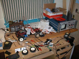
Our Lab at home (we lost so many parts)
|
|
|
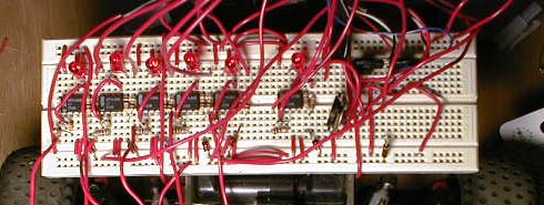
Signal detection circuit