Application Software

Overview

We used the GameX graphics engine to run the main task scheduling loop as well as play-back recorded data in both real time and pre-recorded data sets (.mot files). Microsoft Visual Studio was used to develop this application in C++.

GameX

GameX is a free, open-source game/graphics engine developed by Rama Hoetzlein, a graduate of Cornell University’s Computer Science Department. GameX was designed to provide a single object interface for all game functions, thus eliminating the need to develop sophisticated code using different low-level APIs for sound and graphics. In addition to ease-of-use, GameX is thoroughly documented and comes with extensive demos to support new game developers. [g1]

To import the GameX engine into a Visual Studio project, a few things must be done:

1. The GameX Library, gamex.lib, must be added to the buildable libraries file (check me on this) for the project so it can be build with the project.

2. The Main c++ file must first contain the definition:

#define GAMEX_MAIN

3. The Main c++ file must contain the gamex header file:

#include "gamex.hpp"

4. The Main c++ file must contain three functions: GameInit, GameRun and GameDraw.

A blank main c++ file for GameX is shown below:

// GameX Main C++ File

#define GAMEX_MAIN

#include "gamex.hpp"

void GameInit (void)

{

GameX.Initialize ("Motion Capture", RUN_NOCONFIRMQUIT | VIDEO_32BIT

| VIDEO_WINDOWED | RUN_BACKGROUND, 800, 60

. . .

}

void GameRun (void)

{

. . .

}

void GameDraw (void)

GameX.ClearScreen();

GameX.Begin3Dscene();

. . .

 GameX.End3DScene ();

. . .

}

When compiled and built into an executeable, the program will call GameInit and then consecutively call GameRun followed by GameDraw at a rate of 60 to 70 times a second.

We used the 3D drawing tools in GameX to provide motion capture playback. Some useful GameX objects are:

Vector3DF – A 3D vector containing x,y and z components as 32-bit floating point numbers. These vectors also contain functions to do elementary matrix arithmetic such as normalization, dot product, cross product and scaling.

ImageX – This object represents a 2D or 3D image that can be loaded, constructed and drawn on the screen.

CameraX – This object represents the positioning of a camera in 3D space. These can be manipulated to change the view, angle of view and zoom of the camera.

Point Modeling

To perform motion capture, it was necessary to keep track of the acceleration, velocity, position, and orientation of each of the sensors. This was accomplished in the software using three classes: Point, Elbow, and Wrist. The base class is Point, which contains the variables to keep track of the current sensor state, along with the variables and functions for filtering and averaging. The header of the Point class is shown below:

class Point

{

protected:

Vector3DF offset; // offset value of accelerometer (~183 = 0g)

Vector3DF gravity; // Gravity directional vector

ImageX image; // Image of a single "Dot"

CameraX *cam;

int dist;

int prev_x;

Point *parent; // The point which this point's position

// depends on. ie. the wrist's position

// depends on the elbow's position.

void ForceMove(void);

void LPFilter( Vector3DF &a );

void HPFilter( Vector3DF &v );

float NormalizeAngle(float angle);

float round( float a );

public:

Point();

Point(Vector3DF _pos, int _dist, Point *_parent, CameraX *_cam);

void Run( Vector3DF t, CameraX *c );

void Draw();

void Reset();

Vector3DF pos;

Vector3DF vel;

Vector3DF acc;

float phi, theta, psi;

};

The classes that are directly used are Elbow and Wrist, which are derived from the Point class. They contain redefinitions for the Run(), Draw(), and Reset() functions, since each sensor should affect the position / orientation differently, and of course should be drawn differently since they represent different points on the body. The Elbow and Wrist class header definitions are shown below:

class Elbow : public Point

{

public:

Elbow();

Elbow(Vector3DF _pos, int _dist, Point *_parent, CameraX *_cam);

void Run( Vector3DF t );

void Draw();

private:

};

class Wrist : public Point

{

public:

Wrist();

Wrist(Vector3DF _pos, int _dist, Point *_parent, CameraX *_cam);

void Run( Vector3DF t );

void Draw();

float x_avg;

void Reset();

private:

float avg_vector[NUM_SAMPLES];

int oldest_ptr;

int zero_cnt;

void filter_X(void);

};

The Elbow class determines position and orientation solely by referencing the current measured direction of gravity. The Wrist class determines position and orientation from the current measured direction of gravity, and a numerical integration technique of the rotation acceleration. For a more detailed description, refer to the high level design and the Algorithms section below.

Algorithm

The motion capture point modeling algorithms occur in the Run() functions within the Wrist and Elbow’s classes. In Elbow’s Run function, first an offset is added to the raw acceleration so that the acceleration is 0g centered. The LPFilter function then removes small amplitude accelerations less than a magnitude of 2.0. The phi and theta orientation angles are then calculated according to the formula detailed in the high-level design section. Note that only phi and theta are required to model the body; the velocity and position are relics of an older version that drew the graphics with points and bars, and are retained here for analysis purposes.

void Elbow::Run( Vector3DF rawAcc )

{

Vector3DF prev = pos;

acc = rawAcc - OFFSET;

LPFilter( acc );

float hyp = acc.Length();

phi = atan2( acc.y, acc.z );

theta = asin( acc.x/hyp );

if( theta > 45 )

phi = asin( acc.y/hyp );

vel.x = dist*sin( theta );

vel.y = dist*cos( phi );

vel.z = dist*sin( phi );

pos = parent->pos + vel;

pos.x = vel.x;

phi *= (180/PI);

theta *= (180/PI);

}

The Wrist’s Run function behaves similarly to Elbow’s run function, except with the addition of the filter_X function that applies averaging filters, velocity damping, and numerical integration to determine the psi orientation angle.

void Wrist::Run( Vector3DF rawAcc )

{

// Get the acceleration values by subtracting the DC offset

acc = (rawAcc-OFFSET);

// compute angles

phi = atan2( acc.y, acc.z );

theta = atan2( acc.z, acc.x );

// lowpass filter the acceleration

LPFilter( acc );

// filter x-axis acc further for numerical integration

filter_X();

//psi += acc.x;

// update position based upon angles

pos.x = dist*cos( psi-PI/2 );

pos.y = dist*cos( phi ) + dist*sin( psi );

pos.z = dist*sin( phi );

// set your position based upon your parent's

pos = parent->pos + pos;

// make sure you're always d away from your parent

Vector3DF d = pos - parent->pos;

pos = parent->pos + d*(dist/d.Length());

}

void Wrist::filter_X(){

//---------- Do x-axis DC-blocker ----------//

// implement y[n] = x[n] - x[n-1] + R*y[n-1]

float temp = acc.x; // x[n] value

acc.x = temp - xn_1 + R*yn_1;

// update y[n-1],x[n-1]

yn_1 = acc.x;

xn_1 = temp;

//--------- End DC blocker ----------//

//---------- Do Moving average filter on acceleration ----------//

// update the avg acceleration

// add the newest sample, subtract the oldest sample

x_avg -= avg_vector[oldest_ptr]/NUM_SAMPLES;

avg_vector[oldest_ptr] = acc.x;

x_avg += acc.x/NUM_SAMPLES;

// put the newest sample in the oldest sample spot

avg_vector[oldest_ptr] = acc.x;

// the next element is now the oldest sample

oldest_ptr++;

if( oldest_ptr == NUM_SAMPLES )

oldest_ptr = 0;

//---------- End Filtering acceleration ----------//

//- Magnitude shape the velocity and Do Numerical Integration -//

if( x_avg >= 0.f )

vel.x += log( x_avg+1 )/10;

if( x_avg < 0.0f )

vel.x -= log( -1*x_avg + 1 )/10;

if( -0.01f < vel.x && vel.x < 0.01f )

vel.x = 0;

//--- End Magnitude shape velocity, Num Integration ---//

//---------- Damp the velocity ----------//

if( x_avg > -.4 && x_avg < .4 ){

vel.x *= .1;

zero_cnt++;

}

//---------- End Velocity damping ----------//

//---------- Debounce velocity ----------//

if( vel.x < -.5f && !vel_up ){

vel_down = true;

}else if( vel.x > .5f && !vel_down ){

vel_up = true;

}else if( zero_cnt >= 3 ){

vel_up = false;

vel_down = false;

zero_cnt = 0;

}

if( vel.x > 0 && vel_down )

vel.x = 0;

if( vel.x < 0 && vel_up )

vel.x = 0;

// - numerically integrate the velocity to extract angular position --//

//pos.x += vel.x;

psi += vel.x/dist;

// put bounds on the angle

if( psi <= -PI/2 )

psi = -PI/2;

if( psi >= PI/2 )

psi = PI/2;

}

Serial Port Communication

We used the Microsoft Windows API to interface to the serial port on the computer end. This was accomplished by using built-in Windows functions documented in Microsoft’s MSDN. Using this method supports one of our goals – scalability – in that, the application can then be run on a very wide range computers, using Microsoft Windows 95 to XP and future Windows Operating Systems.

This documentation is available via reference [m1]. Note that this code is easily portable between VB, C, C++, C#, and is similar for other types of hardware ports such as a parallel port (use “LPT1” instead of “COM1”).

Setup:

The interface to the serial port requires inclusion of the windows header file and the global definition of several variables and local (or global) definition of several additional variables for access. The variable definitions are:

// Include the windows header file

#include “windows.h”

// Serial Port Communication Objects

HANDLE hSerialPort;

BYTE Buffer[255];

DWORD BytesRead;

DWORD Success;

DCB MyDCB;

Where:

“windows.h” includes the function calls to the serial port driver as well as object definitions for BYTE (unsigned char), DWORD (unsigned int), HANDLE and DCB.

hSerialPort is a handle (or ID) to the serial port in use. This object is used as a reference to the port when communicating with Windows hardware drivers.

MyDCB is an object that specifies the control settings for a serial communications device.

Buffer is used for physical I/O. The buffer may be of any data format, but will be broken into BYTE-wise format in actual I/O.

BytesRead is a 32-bit integer containing the number of bytes actually read or written to the serial port when an I/O is attempted.

Success is a 32-bit integer returned from any serial port API call, containing the result of the function call (failure, success or any other pertinent information.

Initializing the Port:

Three function calls are required to initialize the serial port for communication. These calls are:

// build serial port handle

hSerialPort = CreateFile("COM1", GENERIC_READ | GENERIC_WRITE, 0, NULL, OPEN_EXISTING, FILE_ATTRIBUTE_NORMAL, NULL);

// set up port parameters

Success = GetCommState(hSerialPort, &MyDCB);

MyDCB.BaudRate = 9600;

MyDCB.ByteSize = 8;

MyDCB.Parity = NOPARITY;

MyDCB.StopBits = ONESTOPBIT;

Success = SetCommState(hSerialPort, &MyDCB);

Where:

Calling CreateFile opens “COM1” for I/O in generic read and generic write modes with normal file attributes (only one program can have control of the port).

Calling GetCommState will give the MyDCB object the properties of the current serial port handle. The DCB parameters are then set for normal RS-232 communication at 9600 baud, with 8 data bites, no parity bits and one stop bit.

Calling SetCommState will then give the serial port handle the properties specified in MyDCB.

Communication:

Both data input and output are simple, requiring only one function call. Reading data is accomplished through:

Success = ReadFile(hSerialPort, Buffer, 255, &BytesRead, NULL);

Where:

The function will attempt to read 255 bytes of data from the computer’s serial port (specified by hSerialPort) into data buffer Buffer and will display the total number of bytes actually read in the variable BytesRead. Note that this function is non-blocking and will read only the number of bytes available in the computer’s serial port buffer.

Writing data is accomplished through:

Success = WriteFile(hSerialPort, Buffer, Buffer.Length, &BytesRead, NULL)

Where:

The function will attempt to write Buffer.Length bytes from Buffer into the computer’s serial port (specified by hSerialPort) buffer and write them out to the port independently. The function will return the number of bytes actually written in BytesRead. Note that this function is also non-blocking as it copies the contents of Buffer into the serial port buffer and the hardware writes the data out independently.

Setting Port Timeouts:

Another important consideration is properly setting the communication port timeouts. If not set properly, calling ReadFile and WriteFile will become blocking functions and unnecessarily consume thousands of CPU cycles. To set the I/O timeouts:

Success = GetCommTimeouts(hSerialPort, MyCommTimeouts);
 
// Modify the properties of MyCommTimeouts as appropriate.
MyCommTimeouts.ReadIntervalTimeout = MAXDWORD;
MyCommTimeouts.ReadTotalTimeoutConstant = 1;
MyCommTimeouts.ReadTotalTimeoutMultiplier = MAXDWORD;
MyCommTimeouts.WriteTotalTimeoutConstant = 0;
MyCommTimeouts.WriteTotalTimeoutMultiplier = 0;
 
// Reconfigure the time-out settings, based on the properties of MyCommTimeouts.

Success = SetCommTimeouts(hSerialPort, MyCommTimeouts);

Where:

MyCommTimeouts is a long pointer to a comm timeouts structure, which has the properties:

ReadIntervalTimeout – Maximum allowable time between bytes being received (in ms)

ReadTotalTimeoutConstant – Total time out period for read operations (in ms)

ReadTotalTimeoutMultiplier – Multiplier for total time out period

WriteTotalTimeoutConstant – Total time out period for write operations (in ms)

WriteTotalTimeoutMultiplier – Multiplier for total time out period

The MSDN states that by setting ReadIntervalTimeout and ReadTotalTimeoutMultiplier to the maximum DWORD (2^32) then when calling a ReadFile, the function will return only what bytes are in the buffer, if there are no bytes in the buffer, it will then block for a single byte recieve, or time out in ReadTotalTimeoutConstant milliseconds. By setting this value to 1, the function will read all bytes, or only block for a total of 1ms. Because a new packet is sent down the data pipe at 100Hz (2.5 ms), then the maximum blocking time will be 1ms, which allows 1.5 ms for running the rest of the code (which is more than enough).

Closing the Port:

The serial port specified by serial port handle can be closed and released by calling:

Success = CloseHandle(hSerialPort)

Error Handling:

In each of these function calls so far, a DWORD result is returned, representing the status of the function call. A simple error handler can be implemented by using these function calls:

if( Success == 1 )

console->Printfn("Comm Port Call Successful.");

else{

// get error and display it

LPVOID lpMsgBuf;

FormatMessage(

FORMAT_MESSAGE_ALLOCATE_BUFFER |

FORMAT_MESSAGE_FROM_SYSTEM |

FORMAT_MESSAGE_IGNORE_INSERTS,

NULL,

GetLastError(),

MAKELANGID(LANG_NEUTRAL, SUBLANG_DEFAULT), // Default language

(LPTSTR) &lpMsgBuf,

0,

NULL

);

console->Printfn("Communication Error: %s", lpMsgBuf );

}

Where:

Success determines the result of the previous call. A value of 1 means a successful call.

FormatMessage is used to get the last error message (GetLastError()) and display it as a string in the natural language of the computer.

LpMsgBuf is a pointer to a message buffer that will contain the error description string.

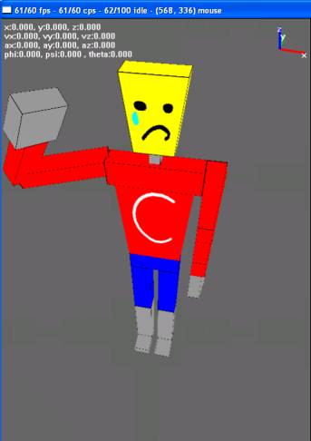
Graphics

The body graphics is drawn using a series of cubic polygons (102 to be exact) and bitmap textured. The implementation is done in the Body class, and as far as the user is concerned, there are only 4 public level functions: Draw, Reset, RotateElbow, and RotateWrist. Reset resets all the angles to the default position, such that the right arm is hanging by the side. The RotateElbow function takes in two parameters, which are the phi and theta orientation angles. RotateWrist takes in the phi and psi orientation angles. Refer to the high level design for the angle definitions. The internal mechanics mostly consists of rotations and transformations of the vertices and more details can be obtained from the code in Appendix A. Figure (14) shows a final screenshot.

Figure (14): Graphics Display Screenshot

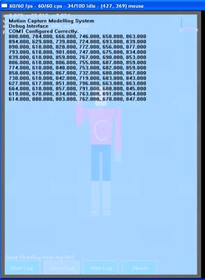
Logging and Playback

The logging and playback feature allows the user to record acceleration data from the microcontroller directly to file and open the file later to replay the corresponding motion in the program. To start logging data, the Start Log button on the lower left corner of the screen is clicked. When the user has finished collecting data, the Save Log button can be clicked to stop logging and save the acceleration log to a user specified file. To playback (run) a log file, the Run Log button is clicked and the user selects a valid log file. The program has been set to disable Run Log while a Start Log is being run and vice versa. The saved log file is text formatted and contains the raw accelerations of the sensors. Hence, the raw data can be exported to external programs such as matlab to perform post analysis or other simulations. A screenshot of loading data is shown below in figure (15).

Figure (15): Data Playback Screenshot

The motion capture logging capability is implemented by the LogFile class whose class header definition is shown below. The data members include a file handle to read and write to a log file, a flag to indicate whether it is in data logging or playback mode and a flag to indicate when it has reached the end of a log file in playback mode.

Opening and Closing a File:

The OpenForWriting and OpenForReading functions take in a file path text string parameter, and open the file for writing or reading respectively. They return true on success and false on failure if the file could not be opened. The Close function closes a file if one is open. This call is required when finished writing the log file.

Printing To and Reading From a Log File:

The Printf function can write formatted text to the log file and returns true on success and returns false otherwise. The function parameters are the same as the standard ANSI-C printf() function, which provide dynamic text formatting capability. To read from a file, the ReadLine() function is called. The input parameter is the character buffer to hold the returned string. ReadLine returns the number of characters read, or –1 if there is an error.

The class header definition is shown below:

class LogFile

{

private:

FILE *accLogFile;

bool writeEn, doneReadingLog;

public:

LogFile();

~LogFile();

bool OpenForWriting(char* fileName);

bool OpenForReading(char* fileName);

void Close();

bool Printf(LPCSTR lpszFormat, ...);

int ReadLine(BYTE buffer[]);

bool IsLogFinished() {return doneReadingLog;};

};

Console

During the development of the software code, there were many instances where we wished we could display status / debugging text out to the screen in a manner similar to a dos command prompt. Hence, we created the Console class, which allowed us to print out useful information, both for us in developing the code and for the user. In addition, the console provides file-logging capability, allowing printouts to the console to be reviewed later in a log file stored on disk. Currently, the console displays error messages and provides a raw print out of the acceleration data obtained from the micro-controller. The “~” button on the keyboard toggles the console on the screen, displaying or hiding the console as necessary. A screenshot is shown below:

Figure (16): Console Screenshot

The Console class structure is shown below:

class Console

{

private:

int x1, x2, y1, y2, maxLines, maxChars;

int locate_x, locate_y;

bool showConsole;

LISTSTR strBuffer;

void NewLine();

void _Print(string newString);

FILE *logFile;

HANDLE hBufferMutex;

DWORD dwWaitResult;

public:

Console();

Console(char* _logFileName, int x1, int y1, int x2, int y2);

~Console();

void SetSize(int x1, int y1, int x2, int y2);

void Printf(LPCSTR lpszFormat, ...);

void _Printf(string newString);

void Printfn(LPCSTR lpszFormat, ...);

void _Printfn(string newString);

void Show() {showConsole = true;};

void Hide() {showConsole = false;};

void Toggle() {showConsole = !showConsole;};

void Draw();

};

To use the console, first a Console object needs to be instantiated. An example is shown below, where printouts to the console are logged to the file “consoleLog.txt”, and the console window will be drawn in the rectangle defined by the two screen coordinate: (10,10) and (500,750).

Console *console;

console = new Console("consoleLog.txt", 10,10,500,750);

Printouts to the screen are now a simple matter of calling the various Print functions provided by the console class. Input strings can be in either Standard Template Library (STL) strings, or standard win32 format strings (ie. “toss in a number: %d”, variableName) the same as those used in the win32 printf function.

console->Printfn("Motion Capture Modeling System");

console->Printfn("Debug Interface");

Refer to Appendix A for code implementation details.

Graphs

Another tool on our wish list during coding and algorithm development was the capability to graph data in real time. The result was the Graph class, which allows the acceleration, velocity, position, orientation, or any other data and its history to be presented on the screen. A screenshot is shown below. This was an indispensable tool in developing the numerical integration algorithm.

Figure (17): Motion Plotting Screenshot

To use the Graphs class, a new Graph instance must first be created. The constructor consists of 7 parameters: the title string, minimum y-axis value, maximum y-axis value, and the 2 points (x1,y1) and (x2,y2) defining the rectangle on screen that the graph is to be drawn on.

accGraph[0] = new Graph("avg_acc1.x", -40, 40, 512, 0, 512+240, 190);

Adding a point to the graph is accomplished by the AddPoint() function that takes in a float argument as the value to be added. The point will be added to the end of the data history list, and if the data list is full the first entry in the list will be removed as the new entry is added.

accGraph[0]->AddPoint(wrist->x_avg);

To clear the entire graph, the ClearAll() function is available, and there are the functions Show(), Hide(), and Toggle to show or hide the graph.

The class header definition is shown below:

class Graph

{

private:

float *ptBuffer;

int *ptScreenBuffer;

int numPoints;

int startIndex;

int nextIndex;

int x1,y1,x2,y2,ymag,xmid,ymid;

int drawDeltaX;

float yaxisMin, yaxisMax, yaxisRange;

float maxSeen, minSeen;

bool showGraph, timeout;

char txt_title[20], txt_ymax[10], txt_ymin[10], txt_xmax[10], txt_minmaxSeen[40];

public:

Graph(string _title, float _yaxisMin, float _yaxisMax, int _x1, int _y1, int _x2, int _y2);

~Graph();

void SetSize(int _x1, int _y1, int _x2, int _y2);

void AddPoint(float pt);

void ClearAll();

void Draw();

void Show() {showGraph = true;};

void Hide() {showGraph = false;};

void Toggle() {showGraph = !showGraph;};

void SetShowGraph(bool _showGraph) {showGraph = _showGraph;};

};