High Level Design

Theory Of Operation

We used our microcontroller to sample and average our accelerometers attached to the body. The data is then transmitted serially to a windows-PC where the data is reconstructed and displayed to the user in real-time.

Motion Capture Math

Overview:

Motion can be captured using several different methods. The two main methods used to extract motion for this project are exploitation of the g-field to observe sensor orientation, and numerical integration to extract change in position. These two options are explored further in the next few sections. First, we will discuss problems to overcome, followed by potential solutions.

In general, the human body has several properties that help constrain motion and help reconstruction of motion from acceleration. Notice that most motion about a joint is rotational. This greatly restricts problems in reconstructing movement because knowledge of how a particular point of the body will move is dependent on the motion type of that point’s parent joint. Moreover, the length of a limb in constant, thus giving a constant radius of movement between joints.

Much of this theory is from reference [a1].

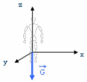
For general purposes, we will define the coordinate system for motion capture as follows:

The Z-Axis will be the up-down axis, which is parallel to the earth’s gravitational field.

The Y-Axis will be facing out from the front of the person.

The X-Axis will be facing out from the side of the person.

This coordinate system is shown below in Figure (1).

Figure (1): Motion Capture Coordinate System [a1]

In the case that the KXM52 is parallel to the Cartesian plane, direct observation of the three outputs (X, Y and Z) will directly reflect the acceleration observed in that direction.

The Dynamic Axis Problem:

One problem with human motion is it is highly non-planar. The result is movement of the accelerometer axes with respect to the motion capture coordinate system. Using 3D-cartesian coordinates in changing axes of measurement can create many undesirable problems. First, if the g-field is considered fixed, a moved axis will pick up accelerations due to g that are not filtered out. Secondly, motion in the moved axis won’t directly represent motion for that point correctly.

Consider the case of an accelerometer measuring acceleration in three orthogonal planes. If the sensor is initially attached to the top of a hand, then the g-field is measured only in the z-axis. Now, if the hand is rotated upwards, a portion of the g-field is observed in both the y and z-axis. If the hand is allowed to rotate 90 degrees, then a portion of the g-field is then observed in both the x and z-axes. These changes will result in a moving gravity vector, as well as dynamic acceleration vectors.

G-Field Observation (Orientation Tracking) Method:

Recall that the KXM52 tri-axis accelerometers used for this project detects both static accelerations, such as the acceleration due to gravity (g) and accelerations due to motion (a). This method makes the assumption that any quick (short-term) acceleration may be disregarded and only DC-accelerations, such as the constant g-field should be observed. This is a relatively valid assumption as the output of the accelerometer is bandwidth limited with a –3dB cutoff frequency of 50Hz.

The orientation of the KXM52 can be uniquely constructed by observing the g-field offset in each axis. If motion in any z-plane is being constructed, then the angle from the normal can be decided.

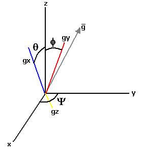
In general, we define three angles in our coordinate system to help with the dynamic movement of axes:

The Normal is defined as the z-axis.

Theta is defined as the angle of the g-field in the xz plane, with respect to the normal.

Phi is defined as the angle of the g-field in the yz plane, with respect to the normal.

Psi is defined as the angle rotation angle of the point in the xy (Cartesian) plane.

These definitions are shown below in Figure (2).

Figure (2): G-Field Component Angles

We can find these angles using simple trigonometry, as shown below in equation (1).

Equation (1): Derivation of G-Component Angles

Using the function atan2(y, x ) in c++ will compute the arctan of y/x in the output range of –p to p [radians]. Thus, human rotational motion can be completely reconstructed because no joints in the body exhibit greater than 360-degree planar rotation about a single point.

Numerical Integration Method:

In cases where there is no G-vector to measure (notably, when the axis of motion is perpendicular to the earth’s gravity vector), one must employ the equations of motion to extract positional changes.

Recall the equations of motion shown below in (2).

Equation (2): Equations of Motion

Using the Euler method, these equations can be approximated by equation (3):

Equation (3): Euler Approximation of Equations of Motion

Taking the small time change (dt) being the sample rate, reduces the equations (in c++ code) to:

Equation (4): C++ Implementation of Euler Approximation of Equations of Motion

v += a;

s += v;

Although this method may seem easier than orientation tracking upon first pass, it is actually substantially more complicated. In this method, the Dynamic Axis Problem is present. Additionally, signal noise will cause substantial jitter to these systems of equations. Because this algorithm computes a running numerical integration, the noise will become additive and can take control of the system entirely. Thus, it is important to develop a filtering system to reduce the noise and allow for proper observation of movement. The next few sections describe our theoretical approach to solve this complicated problem.

Signal Filtering:

An obvious consequence of using long wires and finite precision equipment with limited sampling frequency is noise and error. With respect to numerical integration, finite signal resolution and signal noise can all but destroy a signal’s usefulness. To combat this problem for the numerical integration method, the signals are filtered and band-limited to give more desirable results. The effect can be quite dramatic results. Take for example, the rotational motion of one’s wrist, left and right perpendicular to the earth’s gravitational vector. Obviously, the G-observation method is useless in this case. In figure (3) below, the raw acceleration data is shown as the green plot.

Figure (3): Signal Filtering Methods of Data Lines

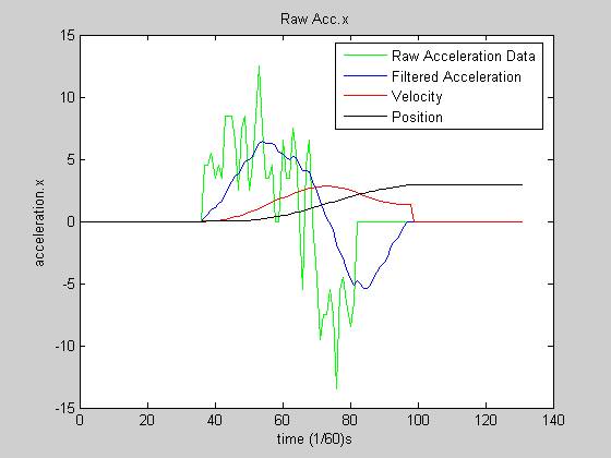
Notice the jitter (quantization error and signal noise) that is inherit to the raw acceleration data. Using a moving average lowpass filter can help destroy much of this noise. Averaging the last N samples together and dividing by N implements such a filter. Expressed in terms of a difference equation, this is:

Equation (5): Moving Average Filter Difference Equation

The result is the blue plot shown above. Notice that there is a small time shift on the output as a result of this filter, while noise immunity is much higher.

Another consequence of both filtering and signal noise is uneven areas for the concave up and concave down humps in the blue waveform. The result, seen through numerical integration of the signal as they velocity (red) plot, is an undesirable DC offset known as drift error. While performing a second numerical integration to extract position (the black plot), the value will drift off to positive or negative infinity. To correct this problem, a small damping term is added into the velocity computation:

1. If the average acceleration is in the range [-.4, .4]

2. Damp the signal by: v = .1*v

Notice how the velocity waveform behaves somewhat appropriately over the range of acceleration, but with some drift term left at the end. The drift is eliminated almost instantly as a result of the damping, once the acceleration settles down. The result on the position plot is a change in position, followed by a constant position.

DC Filtering [f1]:

A final technique required to run our motion capture algorithm requires the DC-filtering of some signals (namely, of a gravity term when necessary). This is implemented using the difference equation:

Equation (6): DC Filtering Difference Equation

With Z-Transform:

Equation (7): Transfer Function of DC Filter

Where R is any constant in the range 0 to 1 (depending on the sampling frequency). The plot below shows the frequency response of the DC Blocking filter, choosing R to be .1.

Figure (4): Frequency Response of DC Blocking Filter

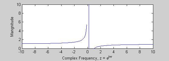
Notice a pole at 0, and a zero about the value 1 (where z=1 corresponds zero frequency). Thus, the filter blocks DC values and preserves the magnitude of higher frequency components. The pole at zero is not a concern as a z-value of zero indicates a frequency component of negative infinity.

This filter is used mostly to combat axes that use numerical integration but do not want to observe acceleration due to gravity.

Magnitude Response:

A final consideration of using numerical integration techniques is the magnitude response of signals. For accelerations of a higher magnitude, the second numerical integral will yield a much grater change in position. The result is the same motion, but at different jerks may yield completely different positional outcomes. To combat this issue, we used a magnitude-shaping filter via the logarithm:

Equation (8): Magnitude Shaping Filter

The result (as seen by figure (5)), is small signals vary linearly (using the approximation that x = log(x) for small x), while larger-magnitude signals become significantly reduced as their magnitude increases. Where the term is used to extract the sign out of the variable x.

Figure (5): Magnitude Shaping Filter Response

Motion Capture Method

We use a combination of both g-field observation and numerical integration to most accurately reconstruct movement through observing acceleration. Both filtering techniques were employed to improve response and accuracy. Our project can model any three-point body system, such as an arm, leg, finger, or hand. We designed a system that holds one point (or joint) of the body stationary and can capture motion of a second joint below. In the case of an arm, the stationary joint is the shoulder, with motion capture running on the arm and forearm. In the case of a leg, the stationary joint is the hip, with motion capture running on the upper and lower leg. The same idea is represented below pictorially:

Figure (6): Motion Capture Tracker Placement

The motion capture trackers can be placed in locations (a), (b), (c), (d) or (e).

In location (a) or (b), G-field observation is used to reconstruct motion on the upper sensor for shoulder to elbow motion. The lower sensor uses G-field observation for y and z motion, and numerical integration and filtering techniques to reconstruct motion in the x-axis. The same holds for locations (e), (d) and (c).