

Roberto Torralbas
& José
Manuel Alvarez
The ![]() project is the first AtMega32 based GPS receiver
( back end) that can track satellites and calculate the navigation solution
from raw digital data.
project is the first AtMega32 based GPS receiver
( back end) that can track satellites and calculate the navigation solution
from raw digital data.
The navigation
solution is the most important goal of GPS design from the view point of the
user. It is calculated by using the observables in a process that involves
solving non-linear equations trough the use of Newton-Raphson technique (later
discussed in this text). Such a navigation solution can be calculated by slow
microprocessors, or even by feeding RINEX2 data) and feeding it to a computer
with a program such as MATLAB. In the Flex Laboratory at
Figure 1. Structure of a GPS receiver by Zarlink using the ARM60 32 bit RISC processor[5].
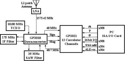
Figure 2.Structure of a GPS receiver using PC ISA I/O Card[6].
In the figures above
one can see three main parts: The RF
Section (GP 2010/2015) , the Correlator
Section (GP 2021), and either the ARM60 Risc Processor (the
microcrontroller) or the PC interface through either ISA or PCI solutions to
implement the Control Section where
the navigation solution is implemented.
In the following sections we will deal with the implementation of the Control Section in the Atmega32
microcontroller.
Rationale:
The GPS WORLD project was inspired in our desire to combine our experience in microcontroller design with our knowledge of GPS theory. Prof. Paul Kintner offered to lend us a very good receiver (DG14) produced by THALES that implements the RF Section, and the Correlator Section. The DG14 is also capable of outputting the raw digital data (from the Correlator Section or GP 2021 chip) through the RS-232 serial communication interface. In past ECE 476 GPS related projects the technology was used to develop many useful and insightful applications, but the fact that through the many years of the course no one had really implemented the technology itself also inspired us to be the first to do it. This of course raised many questions about the capabilities of the Atmega32 microcontroller and how realistic our goal was since we knew the project required high degrees of accuracy and intensive calculations. In the next sections will we show our ups and downs that left to many design decisions which at the end of the day got us a fully functional back end of a receiver.
Background math:
Coordinate transformation:
Once we have calculated the
position of the satellites and our own we need to out put it in a more
comprehensible format. Recall that the calculation were carried out using
Cartesian Earth-Centered-Earth-Fixed (ECEF) X, Y, Z coordinates but the
official reference frame of GPS is the World Geodetic System 1984 (WGS-84)
latitude (![]() ), longitude (
), longitude (![]() ), and altitude(
), and altitude(![]() ). This section explains the transformations which our
project undertakes when representing the GPS results in ellipsoidal coordinates
from Cartesian coordinates.
). This section explains the transformations which our
project undertakes when representing the GPS results in ellipsoidal coordinates
from Cartesian coordinates.
Given the (X, Y, Z)ECEF
the longitude (in degrees) may be calculated using the following equation: ![]() . For the other two components an iterative approach is
necessary since the latitude and altitude values depend on each other. First calculate the radius of a parallel:
. For the other two components an iterative approach is
necessary since the latitude and altitude values depend on each other. First calculate the radius of a parallel: ![]() , and approximate an initial latitude:
, and approximate an initial latitude:  , where e2 = 0.00669437998863492 is the square of
the Earth’s orbital eccentricity.
, where e2 = 0.00669437998863492 is the square of
the Earth’s orbital eccentricity.
1. Compute an
approximate radius of curvature:  ,
,
where a = 6378137.00000 m and b = 6356752.31425 m are the semi-major and semi-minor axis of the reference ellipsoid respectively
2. Compute
the height: ![]()
3. Compute
the new latitude: 
4. If ![]() (where epsilon is a
very small number) then the loop ends otherwise set
(where epsilon is a
very small number) then the loop ends otherwise set ![]() and repeat step 1
through 3.
and repeat step 1
through 3.
For
more on coordinate transformation of GPS results please see Chapter 10 of GPS:
Theory and Practice by B. Hofmann-Wellenhof. To see the algorithm in C refer to
the latlong() function in gpc.c
Newton-Raphson
Method:
The Newton-Raphson method is an
interactive technique for finding roots of a nonlinear function that are well
behaved (their derivatives can be obtained easily). During the process of
obtaining the navigation solution this method will be used, but for now we will
show only the mathematical theory that in a future section will allow better
understanding of the code implemented. If you desired to look at the one
dimensional case you can look it up in any Calculus book, but we will jump
right in to the multidimensional case since is the one that applies to the
navigation solution. The Newton-Raphson
method is based on the Taylor Series expansion and for the case of three
variable function such Taylor Series can be written in the form:
![]()
where ![]() are the roots of
are the roots of![]() and
and ![]() are the guesses at the root. Our whole goal in this case is
to obtain a solution for
are the guesses at the root. Our whole goal in this case is
to obtain a solution for ![]() ,
,![]() ,and
,and ![]() . Since
. Since ![]() ,
,![]() ,and
,and ![]() are essentially three
variables( say
are essentially three
variables( say ![]() respectively) in order to solve for theme we need three
independent equations:
respectively) in order to solve for theme we need three
independent equations:
![]()
![]()
![]()
The hardest part theoretically is
finding the independent equations since after that the problem can be solved
with some basic linear algebra. For example say :
 ,
,  , and
, and  then we can rewrite
our system of equations in the from:
then we can rewrite
our system of equations in the from:
![]() which has the solution
which has the solution
![]() . The equations are
then iterated using the new guesses
. The equations are
then iterated using the new guesses![]() ,
, ![]() ,and
,and![]()
To
see the algorithm in C refer to the solvePos() function
in gpc.c.
Gauss-Jordan
Elimination:
Solving a system
of linear equations using MATLAB or even by hand is one thing and with a
microcontroller is another. When it came
to solving ![]() for a system of four equations and four unknowns our design
choice was the Gauss-Jordan elimination method. Most academics are very likely
to suggest not to use Gauss-Jordan elimination method and instead to go with a
variant like LU decomposition. There are good reasons why you might not want to
use Gauss-Jordan elimination since it requires all the right-hand sides to be
stored and manipulated at the same time, and is significantly slower than LU
decomposition. Nevertheless the Gauss-Jordan method is very straightforward,
and easily to understand, and for these reasons we chose to implement it in
this version of the project .We recommend using another linear-equation solver
in further developments of the project. That being set lets look over the mathematics.
for a system of four equations and four unknowns our design
choice was the Gauss-Jordan elimination method. Most academics are very likely
to suggest not to use Gauss-Jordan elimination method and instead to go with a
variant like LU decomposition. There are good reasons why you might not want to
use Gauss-Jordan elimination since it requires all the right-hand sides to be
stored and manipulated at the same time, and is significantly slower than LU
decomposition. Nevertheless the Gauss-Jordan method is very straightforward,
and easily to understand, and for these reasons we chose to implement it in
this version of the project .We recommend using another linear-equation solver
in further developments of the project. That being set lets look over the mathematics.
Say
you want to solve ![]() :
:

![]() =-
=-
Compose an augmented matrix with the right hand side of the equation above

Now, perform elementary row operations to put the
augmented matrix into the upper triangular form

Solve the equation of the kth row for ![]() (for the three dimensional case k=3 at the beginning), then substitute back into the equation of the k-1th
row to obtain the solution for
(for the three dimensional case k=3 at the beginning), then substitute back into the equation of the k-1th
row to obtain the solution for ![]() an continue until you solve for all
an continue until you solve for all
![]() . This can be written mathematically as follows:
. This can be written mathematically as follows:

To
see the algorithm in C refer to the solvePos() function
in gpc.c
Orbital Dynamics:
In this section we discuss the orbits of GPS satellites and a very high level explanation of what the code in function FindSat() in gp.c accomplishes. If the reader desires a deeper explanation here we take the opportunity to refer him to a good physics book that explains the gravitational attraction between two points with given masses and to GPS: Theory and Practice by B. Hofmann-Wellenhof.
Figure 3 An elliptical orbit in the orbital coordinate frame(x0,y0).
This is the shape of a satellite orbit and could be also
described by equation  where
where ![]() is a constant for a
specific orbit (not discussed here) and e
is the orbital eccentricity (if e
< 1 then the orbit is elliptical, if e
= 1 then the orbit is circular). It turns out that there is a relation between
the parameters a, e and
is a constant for a
specific orbit (not discussed here) and e
is the orbital eccentricity (if e
< 1 then the orbit is elliptical, if e
= 1 then the orbit is circular). It turns out that there is a relation between
the parameters a, e and![]() :
:
 ,
,  ,
, ![]() ,
,
meaning we can figure out
![]() given a and e or vice versa. Hence we only need two parameters to determine the
shape of the orbit. We will use a and e
(which are two of the required six
ephemerides in order to know the satellites position) in FindSat()
function in gps.c .
given a and e or vice versa. Hence we only need two parameters to determine the
shape of the orbit. We will use a and e
(which are two of the required six
ephemerides in order to know the satellites position) in FindSat()
function in gps.c .
Once we know the shape of the satellite then it is necessary to orient it in space as shown in Figure 4.
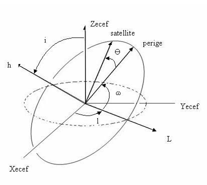
Figure 4.Orbital parameters specifying a satellite position.
The extra parameters needed to orient the satellite are the inclination (i, usually around 55 degrees for all satellites), the longitude of ascending node (l), and the argument of perigee (ω).The final parameter necessary to calculate the position of the satellite is the true anomaly Ө. If we know the true anomaly we can find the satellite and no more calculations are necessary. Of course it is not that simple because the true anomaly is sent every four hours with the rest of the ephemerides implying we can only calculate the exact position for each satellite every four hours. This is not what we want but we will leave this discussion of how to calculate Ө and orbital time dependence for a future section in this text(Program/Hardware Design). Nevertheless there is a step that even though we are not going to explain in detail should be mention (carefully explained in GPS: Theory and Practice by B. Hofmann-Wellenhof). Once we use the ephemerides we know the orientation of the orbital plane with respect to the ECEF coordinate. This is grea,t but what we really want is the satellite position with respect to earth and not its own orbital plane (Xorb ,Yorb, and Zorb) as shown in Figure 3. Therefore we do some simple transformation, rotating about the needed axis to get the ECEF coordinates for each satellite. This can all be seen in the last lines of FindSat() procedure in gps.c. The complete transformation consists of multiplying three rotational matrixes:

where ![]() are rotation matrices
and refer to the axis labeled in Figure 4. Meaning we first rotate around h,
then l, and finally z axis (notice that the order of the rotations affects the
result).
are rotation matrices
and refer to the axis labeled in Figure 4. Meaning we first rotate around h,
then l, and finally z axis (notice that the order of the rotations affects the
result).
Logical Structure:
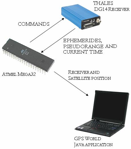
Figure 5: High-level design structure
Instruments:
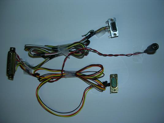
Figure 6: RS 232 serial converter...
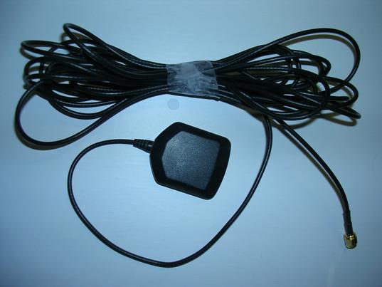
Figure 7: ACC GPS antenna, model GPS-P1MAM
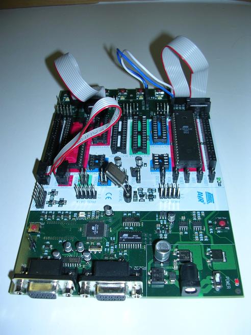
Figure 8: STK500 with ATMega32
microprocessor.
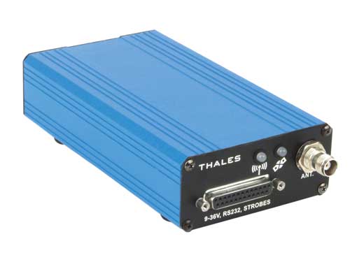
Figure 9: THALES DG14 receiver
Extracting Raw Satellite Data:
The orbital
ephemerides are calculated very accurately as part of the GPS control segment
up-linked to the spacecraft about once per day and updated in the navigation
message about every 4 hours. To convey these parameters to the user, they are
encoded on the GPS C/A (civilian access) signal so that each satellite transmits
its own orbital parameters. GPS receivers like the THALES DG14, acquire and
store these parameters to calculate their own location and that of the
satellites which they are tracking. To obtain raw ephemerid data the MCU sends
the appropriate SNV command through Port B using the GetEphem() function. This function makes the receiver
execute the following command: $PASHQ,SNV,A. This command queries for ephemeris data
from each satellite currently being tracked by the receiver, and outputs the
response through Port A. The SNV message response has the following format: $PASHQ,SNV,<Ephemeris
data string + checksum>. The ParseEphem() function then takes care of breaking down
that response message whose structure is summarized in table below. Note that
the first 11 characters in this message ($PASHQ, SNV,) are discarded by the parser.
Table 1: SNV Response message structure
|
Field |
Bytes |
Content |
|
short wn |
2 |
GPS week number |
|
long tow |
4 |
Seconds of GPS week |
|
float tgd |
4 |
Group delay (seconds) |
|
long aodc |
4 |
Clock data issue |
|
long toc |
4 |
Clock data reference time in
seconds |
|
float af2 |
4 |
Satellite clock correction (s/s2) |
|
float af1 |
4 |
Satellite clock correction (s/s) |
|
float af0 |
4 |
Satellite clock correction (s) |
|
long aode |
4 |
Orbit data issue |
|
float deltan |
4 |
Mean anomaly correction (semicircles/s) |
|
double m0 |
8 |
Mean anomaly at reference time (semicircles) |
|
double e |
8 |
Eccentricity |
|
double roota |
8 |
Square root of semi-major axis (m1/2) |
|
long toe |
4 |
Reference time for orbit or time of epoch (s) |
|
float cic |
4 |
Inclination cosine harmonic correction (rad) |
|
float crc |
4 |
Orbit radius cosine harmonic correction (m) |
|
float cis |
4 |
Inclination sine harmonic correction (rad) |
|
float
crs |
4 |
Orbit radius sine harmonic correction (m) |
|
float cuc |
4 |
Latitude cosine harmonic correction (rad) |
|
float cus |
4 |
Latitude sine harmonic correction (rad) |
|
double omega0 |
8 |
Longitude of ascending node (semicircles) |
|
double
omega |
8 |
Argument of perigee (semicircles) |
|
double i0 |
8 |
Inclination angle (semicircles) |
|
float omegadot |
4 |
Rate of ascension (semicircles/s) |
|
float idot |
4 |
Rate of inclination (semicircles/s) |
|
short accuracy |
2 |
User range accuracy |
|
short health |
2 |
Satellite health |
|
short fit |
2 |
Curve fit interval |
|
char PRN |
1 |
Satellite PRN number minus 1 (0 to 31) |
|
char
res |
1 |
Reserved character |
|
checksum |
2 |
--- |
Depending on the data type of each
parameter the parser will call different special data reading sub functions
like ReadLong(), ReadFloat(), ReadShort(), and ReadDouble(). The later was particularly more difficult
to implement and hence we have dedicated the next subsection to document this
special case. One last crucial parameter which needed to be extracted for our
calculation was the time at which the signal was received. The GetCurrentTime() function accomplishes this task by sending
the following command to the receiver: $PASHQ,XYZ,A. This command queries the three-dimensional position for each tracked
satellite, outputting the response through Port A. The table below outlines the
structure of the response message. Notice that rows three to seven of this
table repeat themselves in the response message depending on the total number
of satellites being tracked by the receiver. The ParseCurrentTime() function which reads this output also stores
the satellite locations coordinates to compare the calculation made by the to
our own. The data is later sent to the GPS WORLD Java application to be
displayed and compared.
Table 2: XYZ Data String
|
Field |
Bytes |
Content |
|
long[RcvTime] |
4 |
Time at which the signal was
received in milliseconds of the week referred to GPS system time. |
|
short [Total Satellites] |
2 |
The total number of satellites
appearing in the message. |
|
short [sv_n] |
2 |
The PRN number of the satellite
(being tracked on channel n of the DG14 |
|
double [satx_n] |
8 |
The x coordinate of the satellite
being tracked on channel n of the DG14 |
|
double [saty_n] |
8 |
The y coordinate of the satellite
being tracked on channel n of the DG14 |
|
double [satz_n] |
8 |
The z coordinate of the satellite
being tracked on channel n of the DG14 |
|
double [range_n] |
8 |
The corrected pseudo-range of the
satellite referenced in [sv_n] |
|
checksum |
2 |
--- |
Double to Single Precision Float
Conversion:
One of the
many challenges that arouse right as we were extracting the raw satellite data
was that some of the ephemeris parameters which the THALES DG14 receiver sent
out were double precision floats (64 bit) while the Code Vision AVR is
restricted to single precision (32 bit) floating point arithmetic. This meant
that unlike the other parameters which were easily parsed using the methods of
the previous subsection these ephemerides needed to be converted before we
could use them. For this conversion of raw, unformatted or “binary” data we
first consulted the IEEE standard for floating point arithmetic.
The IEEE single precision floating point number consists of a sign bit (S),
followed by eight exponent bits (E), the 32 bit word is completed by 23
fraction (F) bits (see Figure 10). The IEEE double precision floating point on
the other hand consist also of a sign bit (S), but it’s followed by eleven
exponent bits (E), this 64 bit word representation is completed by 52 fraction
(F) bits (see Figure 11).

Figure 10: IEEE single precision floating point representation

Figure 11: IEEE double precision floating point representation
The ReadDouble() function takes care of the conversion which begins by parsing the 64 bit word character by character using the getchar() function in Code Vision AVR and storing those in temporary double_buffer eight element unsigned character array. Since our target is to have a 32 bit word in the end, the first element of this array (double_buffer[0]) is casted into an unsigned long format and shifted left by 24 bits to move the original eight bits to the beginning of the word. AND’ing the result with 0b10000000000000000000000000000000 guarantees that the new word consists only of the S bit followed by 31 zeros; lets call this new word S. Converting the exponent bits of the floating point value is a quite more complex. For the exponent section for example we first have to look into the first and second elements of the double_buffer array and shift those around so as to leave only the exponent bits in an unsigned int format (see Figure 12 below). But notice that we still have eleven exponent bits and the single precision float must have only eight. This final conversion is achieved by subtracting 1023 and adding 127 to offset the value leaving only eight 0 bits followed by eight exponent bits. This result is then casted into a 32 bit unsigned long format, and shifted left by 23 bits to set the bit in the correct position. We call this new word E.
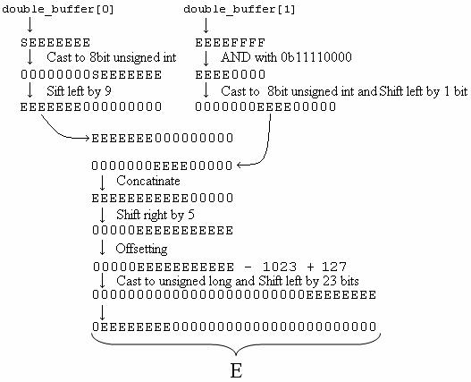
Figure 12: Single precision floating point Exponent bits
To convert the fraction bits we simple took the first 23 of the original 52 bits in the double precision fraction bits. To do this we needed to look into the second, third, fourth and fifth elements of double_buffer array which as you may recall contains the raw double precision float bits. The values are assigned to temporary variables and casted into unsigned long format and later shifted left by 28, 20, 16, and 4, respectively (see Figure 13 below). These four 32 bit words are then concatenated and to guarantee that only the most significant 23 bits are used we AND the result of the concatenation with 0b11111111111111111111111000000000. Finally, to set the bits in the correct position we shift the bits in this new F word to the right by 9.
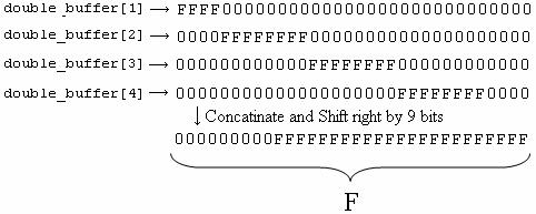
Figure 13: Single precision float fraction bits
The S, E, and F words are then concatenated to obtain the single precision floating point value V.
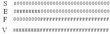
Figure 14: Single precision float complete bit representation
Satellite Tracking:
Figure 15 shows a screenshot of the Java application developed by Roberto Torralbas that was used to display satellites on a world map. The program consist of tabs to also allow display of some of the raw data extracted (ephemerides, pseudoranges) and the calculated satellite coordinates as well as the navigation solution. Notice that in the screenshot there are two markers ( white ,and red) of different colors currently tracking satellite 6 and 26. Satellite 6 is the one we calculated/extrapolated the true anomaly for every second from the TOE (time at which ephemeris were sent). Satellite 26 we are given the ECEF coordinate by the DG14 receiver and the pseudoranges and is the one we use to calculate the navigational solution. The reason for using satellites for which we are given their ECEF coordinates instead of those which we calculate ourselves is because the receiver only give pseudoranges for those which it believes to have a good reading. This caused for us not to have pseudoranges for some of the satellites positions we were calculating and therefore had to use their calculations which came with the corresponding pseudoranges.
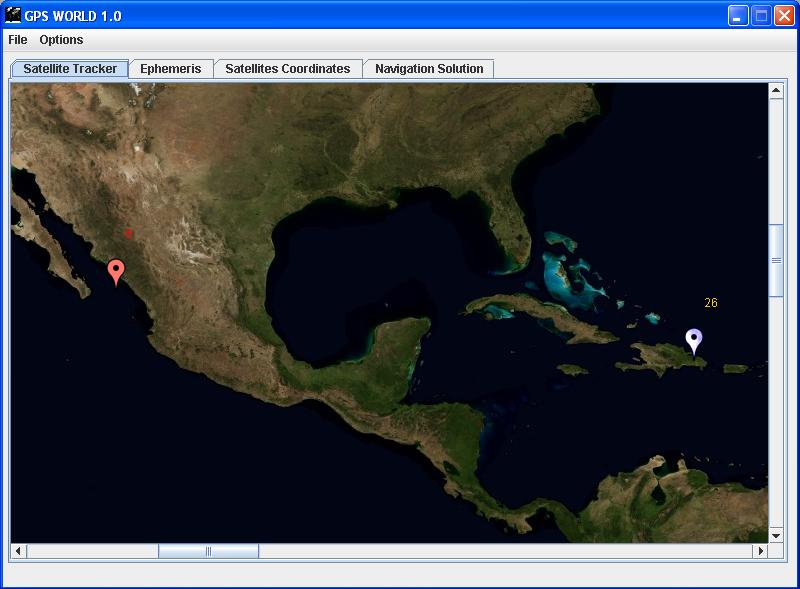
Figure 15.Screen shot of the GPS WOLD GUI developed in Java
Here is a short film of one satellite moving in the map. We are updating the satellite calculation about every second.
We will not enter in detail of the implementation of the user interface in Java, but if interested in writing your own , please refer to www.sun.com, and make sure you look up the javax.comm API so that you are able to connected serially to the microcontroller. Essentially the application serves as a custom, sophisticated version of HyperTerminal.
That being said lets move on to explain how the True Anomaly θ is calculated for times after the TOE (time at which the ephemeris were sent). The problem arises with the elliptical shape of the orbit, which does not allow the True Anomaly to be calculated as trivially is if we were dealing with circular orbit (for which the True Anomaly would had been a linear function of time). The challenge is to derive equation of motion to determine the time dependence of a satellite within its orbit. This was done in FindSat() and here we refer the reader to GPS: Theory and Practice by B. Hofmann-Wellenhof to see more of the theory as its beyond the scope of this paper to explain terms such as Mean Anomaly and Eccentric Anomaly which are used to derive the equations of motion.
Navigation Solution:
Once the
ephemerides and the pseudorange have been extracted for every satellite (and we
know the ECEF coordinates for at least four satellites) it is time to calculate
the navigation solution. The technique implemented in this project is based on
the code range determined by pseudoranges. By the code range we mean the
pseudorange obtained at a known time tagged as the receiver time. The
pseudorange from satellite j to the
receiver measured at time t is![]() . The pseudo range may be represented mathematically as:
. The pseudo range may be represented mathematically as: ![]() , where
, where![]() is the satellite clock offset (obtained from the satellites
along with the ephemerides),
is the satellite clock offset (obtained from the satellites
along with the ephemerides), ![]() is the receiver clock offset (unknown), and
is the receiver clock offset (unknown), and ![]() is the actual range.
The later is the true distance from the jth
satellite at
is the actual range.
The later is the true distance from the jth
satellite at ![]() to the receiver
at
to the receiver
at ![]() , or just simply:
, or just simply: ![]() . If we plug the equation for the true range into that of the
pseudo range and rearrange it so that the left side has the known measured
values and the four unknown values X, Y, Z,
. If we plug the equation for the true range into that of the
pseudo range and rearrange it so that the left side has the known measured
values and the four unknown values X, Y, Z, ![]() are on the right then
we are left with:
are on the right then
we are left with:
![]() .
.
Since we have one equation like
this for every satellite that we are tracking then we only need to track four
satellites to have four equations and hence solve for our four unknowns. The
Newton-Raphson method which we previously explained was used to solve the
equation above. We first chose an initial guess ![]() which differs from the
true position by
which differs from the
true position by ![]() . We need to calculate these differences in order to correct
this initial guess as to approach the true position. We begin by performing a
first-order
. We need to calculate these differences in order to correct
this initial guess as to approach the true position. We begin by performing a
first-order  , where
 ![]() is the initial guess for the actual range. This equation is
then substituted into that of the pseudorange and rearranged (moving all known
value to the left and leaving the unknowns on the right) to obtain:
is the initial guess for the actual range. This equation is
then substituted into that of the pseudorange and rearranged (moving all known
value to the left and leaving the unknowns on the right) to obtain:
 ,
,
where the derivatives
(calculated at the initial guess) are given by: ![]() . Given that we need four satellite (hence four sets of
equations) to solve for the four unknowns it is most convenient to use the
following matrix notation:
. Given that we need four satellite (hence four sets of
equations) to solve for the four unknowns it is most convenient to use the
following matrix notation:
This linear system has a
solution ![]() which is calculated
using the Gauss-Jordan Elimination method which we described earlier. The
differences are then added to the initial guess to calculate de actual
position. To improve the accuracy of this method it must be repeated several
times, and at each point the previous actual position becomes the new guess
position.
which is calculated
using the Gauss-Jordan Elimination method which we described earlier. The
differences are then added to the initial guess to calculate de actual
position. To improve the accuracy of this method it must be repeated several
times, and at each point the previous actual position becomes the new guess
position.
MCU Serial Communication:
To implement serial communication on the Mega32, we referred to the ECE476 serial page. Essentially all we do is set up the UART by turning on the transmitter and receiver(UCSRB = 0b00011000). We set UBRRL to 103 to set the baud rate to 9600, which is the baud rate at which the DG14 transmits data by default. We also found convenient to turn on the receiver and transmitter at the beginning of every iteration ( allowing to send commands to the DG14 and the Java application, and turning it off at the end of the iteration which clears the receiver buffer just in case the DG14 was sending some extra information we did not want to parse(otherwise in the next iteration the program could parse incorrectly).
The serial connections that we made with some wires and connectors recycled from old cables is shown in Figure 16. In case the reader is wondering what is going on, the DG14 assumes that the connections specified in page 13 of the manual are going to a null modem cable. We took a shortcut and implemented the null modem cable between the DB25 and the DB9 connectors
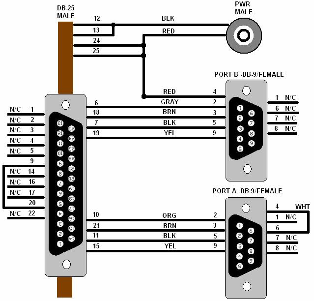
Figure 16: DG14 Receiver Power-I/O
Connections
In order to verify the accuracy of
our calculations we connected our receiver to antenna #2 in the Flex Laboratory
(Phillips hall,
![]() ,
,
which turned out to be approximately 123 meters.
This result was quite satisfactory given that we did not account for ionospheric corrections, and that the floating point conversion may have reduced the accuracy in the data. This result gives us a ball park estimate of the error give or take a few hundred meters. This is satisfactory because with the given complexity of the project and the many challenges that we overcome is almost a miracle that we were this close.
The GPS World project met all specification we set out to do when we first wrote the proposal. It tracks satellites with a very small error in their position and it calculates a three dimensional navigation solution( altitude, latitude, and longitude) within a reasonable error given the single precision floating point problem and the many corrections that could still be implemented in further development of the project. It is too early into the project to consider any patents, as it is difficult to compete with large companies that have been implementing receivers for many years now, nevertheless the project leaves much room for improvement and future developments.
Further Developments:
1-) Lost of debugging and testing. This being a first version it is sure to have a couple of bugs here and there. We actually recommend that before implementing the next version of GPS World to test and verify that all errors are due to hardware/software limitations( double vs single precision floating point) and not programming errors or conceptual ones, like making sure leap seconds are accounted for which we believe to have done (13 seconds), but later found out it has changed to 14 leap seconds by GPS standards.
2-) Currently we are using four satellites ( the first four the DG14 locks on with available pseudoranges) to compute the navigation solution. Using the over-determined solution which involves using 4 or more satellites to calculate the navigation solution is sure to improve the accuracy on most of the cases.
3-) Ionespheric corrections where not implemented and this could also improve the accuracy by a couple of meters or more.
4-) Our linear equation solver uses Gauss-Jordan Elimination method and it could be changed to one more efficient using the LU decomposition method. This may improve on the memory usage which can be a big factor when calculating the over determined solution.
6-) A more ambitious goal would be to try to develop the whole receiver now that you know the back end works. Having the Atmega32 communicating with the GP2021 should be an challenging task that by no means looks impossible to accomplish.
7-) Develop a velocity solution.
As one could see the list could keep on expanding as far as imagination allows it, and that’s great!
Intellectual Property and
Legal Considerations:
Nowadays GPS technology is everywhere, and society becomes more dependent on it everyday. Right now this project serves mainly as an educational tool that should not be integrated to any other appliance that may be of value to you as there has not been enough testing. As an educational tool we expect other students to feel free to expand on this and encourage them to build on and re-use our code as long as proper credit is given to the initial creators: Roberto Torralbas and José Manuel Alvarez.
What is captivating about GPS WORLD is that
it’s an academic (non-for-profit) project which accomplishes all that same
things that expensive commercial receiver do, by using a simple ATMega32
microcontroller, instead of a more powerful chip. Hence, our venture does not violate on any
copyright laws or patents since it constitutes a new solution to a common
problem. When it comes to legal considerations is hard to find ways in which
our little project could violate any. All the code was implemented from our
knowledge of classes such as ECE 415 offered by Prof. Kintner at
The IEEE Code of Ethics referenced below was followed during the design and implementation of this project:
- to accept responsibility in making decisions consistent with the safety, health and welfare of the public, and to disclose promptly factors that might endanger the public or the environment;
All decisions made during the design and implementations of this project were done responsibly and looking after the safety, health, and welfare of the public. The final product hence presents no eminent danger to the public, but will be handle with great care in case that some endangering factors arise in the future.
- to avoid real or perceived conflicts of interest whenever possible, and to disclose them to affected parties when they do exist;
We believe that are no conflicts of interest, and hence no affected parties.
- to be honest and realistic in stating claims or estimates based on available data;
All claims made and detailed throughout this report have been shown to both theory and practice.
- to reject bribery in all its forms;
This is an academic non-for-profit project and no bribery issues arouse at any point during the design or implementation of it.
- to improve the understanding of technology, its appropriate application, and potential consequences;
We hope that our project will help in the understanding of GPS theory ad application, and its many capabilities.
- to maintain and improve our technical competence and to undertake technological tasks for others only if qualified by training or experience, or after full disclosure of pertinent limitations;
Both team members have taken introductory and advance GPS
theory, implementation and receiver design courses at
- to seek, accept, and offer honest criticism of technical work, to acknowledge and correct errors, and to credit properly the contributions of others;
Critiques and suggestions by Prof. Bruce Land and the other ECE 476 labs TAs have been well received and greatly appreciated by our group. We also appreciated the help provided by Prof. Paul Kintner and (PhD) Alex Cerruti regarding GPS receiver specifics.
- to treat fairly all persons regardless of such factors as race, religion, gender, disability, age, or national origin;
Both team members have sustain all common ethical considerations regarding each other as well as members from other teams, teaching assistants, professor, and any other personnel involved in this project.
- to avoid injuring others, their property, reputation, or employment by false or malicious action;
Both members watched over the well-being of others and their property during the course of this project.
- to assist colleagues and co-workers in their professional development and to support them in following this code of ethics.
Our team has and will continue to provide support to our peers in their professional and social endeavors.
Acknowledgment
We want to thank Prof. Paul Kintner, and Alex Cerruti (PhD candidate) for all teaching us GPS theory with great dedication and letting us use their DG14 receiver.
Also we want to thank Prof Bruce Land for all his help during the course , his dedication to teaching, and letting us embark on this ambitious goal.
Code:
- constants.h (header file with constants used)
- gps.c (CodeVision
C program for programming Mega32)
Pictures:
Figure
17:
Parts:
|
Part |
Cost |
Supplier
|
|
ATMega32 |
$8.00 |
ECE 476 Lab |
|
Custom PC board |
$5.00 |
ECE 476 Lab |
|
ATMEL STK500 |
$15.00 |
ECE 476 Lab |
|
THALES DG14 Receiver |
Free |
Prof. Paul Kintner |
|
ACC GPS Antenna (model GPS-P1MAM) |
Free |
Prof. Paul Kintner |
|
RS-232 Connectors (1 DB25 male and 2 DB9 female) |
Free |
Spare Parts |
|
Total |
$32.00 |
|
Work Distribution:
All tasks except the Java application (Roberto Torralbas) were carried out by both team members in the ECE 476 lab and the home-made lab room we created.
References
Datasheets:
[2] THALES DG14
Used
images:
[3] Blue Marble (for high resolution world map)
[4] Google Maps (for marker images)
[5] Zarlink (Receiver structure)
[6] Zarlink (PC ISA I/O Card)
Background Sites:
[7] ECE 476 AVR serial communication