PIC-32 Markov Chain Music Synthesizer
By Rishi Singhal, Raghav Kumar, and William Salcedo
For our final project, we attempted to use the PIC32 as a music player that generated new, coherent music based on the variety of Midi files taken as input. The PIC32 played music via the DAC, based on several Markov chains that stored note probabilities in their respective transition matrices. These transition matrices, in turn, were populated during the training process.
We divided our project into two distinct parts - the computationally intensive, training part that ran on the desktop PC and the music generation part that ran on the PIC. We decided to offload the training process to the PC because processing the large number of Midi files required memory that exceeded the PIC’s capacity.
The training code was written in Python and once the training process was completed, we would copy over the transition matrices to the PIC which would then take care of executing the notes as per the probability transitions.
Our biggest inspiration for this project was the Boids lab wherein we enjoyed the experience of changing external parameters only to be surprised by the random, and often pleasant looking patterns that the PIC produced on the TFT. We aimed to do something similar, only with music as we hoped that each time we ran our algorithm, random yet coherent music would be played by the PIC. The output would vary not just due to the inherent randomness of our algorithm but also due to our ability to change the training music and vary the instruments.
In addition to our interest in random music generation, we were further inspired to work on this project after running Bruce Land’s FM synthesis code and really enjoying hearing the result. Using FM synthesis, his algorithm was already able to play different notes on a scale, beats and instruments. By extending his work, we were able to add chords and generate songs using Markov chains.
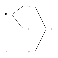
Markov chains were the backbone of our algorithm. As seen by the diagram on the left, a Markov chain is essentially like a Finite State Machine where the state transitions are based on probabilities instead of some conditionals. The matrix on the right is how we represented our various Markov chains. Each row in this matrix holds the probability of going from a certain state to another. For example, the first row represents the probability of transitioning from state A to itself (0), to state B (0.1) and to state C (0.9). Similarly, the second row contains the same probabilities for state B.
Figure 1: The Markov chain and Transition Matrix
When implementing our Markov chains to generate music, it was important to evaluate the tradeoff between memory and quality of music. Having a higher order Markov chain leads to higher quality music as it would retain longer sequences of notes and durations and train based on this longer stretch of data, but this also uses more memory. Lower order Markov chains are lower in memory, but this means the music will be trained based on less sequences of notes such as the last one or 2 notes rather than the last 3 or 4 notes. In our previous plan of encoding notes, we would have 36 different notes stored, corresponding to 36 frequencies. But this soon became problematic as a second order Markov chain would be 36x36x36 bytes, or 46.656 kilobytes. This is a large amount of memory usage and thus we needed to either lower the octaves— which is undesirable since it restricts the notes we can play from, lower the order— also undesirable since it would allow a lot more randomness to be trained in the algorithm rather than distinct patterns, or find another way. To resolve this problem and overcome this tradeoff, we changed the structure of how we decide our notes. Rather than having a large chain of 36 notes, we separated it into 2 different chains: a chain to pick one of four octaves and a chain to pick one of 12 semitones within an octave. This allowed us to have higher order chains with less of a memory cost since this was now broken down and our algorithm can take our octave plus our note offset to figure the actual frequency we want to play.
In our algorithm, we had three primary Markov chains and two secondary Markov chains that depended on the primary chains. The three primary chains were as follow -
The PIC-32 has been programmed with a frequency-modulation synthesis algorithm created by Professor Bruce Land. FM Synthesis is a digital synthesis method where the output synthesis frequency is modulated. In our implementation, note frequencies were mapped to integer values so they work with the discrete nature of Markov chains.
FM synthesis is critical for our project because it allows for a more unique and pleasant sounding output sound for the PIC-32. This method of audio synthesis allows simulation of sounds such as plucked strings, marimbas, and even a guitar.
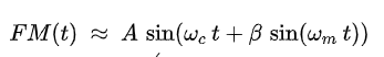
From a high level this method of synthesis makes use of this general formula:
Figure 2: FM Synthesis Equation(sourced from https://en.wikipedia.org/wiki/Frequency_modulation_synthesis)
This formula is implemented using the sine-table synthesis algorithm, and every timestep this formula is computed and output by the DAC. Another important implication of this implementation is a differential-equation based amplitude envelope function. Because we are using an interrupt we used the discrete time nature to calculate the differential equation “on the fly.” The FM synthesis algorithm calculates two differential equations for the amplitude envelope, one for  and one for
  .
.
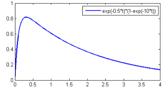
Figure 3: Differential-Equation Based Frequency Envelope
(sourced from https://people.ece.cornell.edu/land/courses/ece4760/PIC32/index_sound_synth.html)
Figure 3 shows a sample differential equation solution based on certain inputs.To calculated this efficiently in a discrete-time manner, the solution is simplified to y(n)=y(n-1)*R.
It is no secret that, like most microcontrollers, the PIC-32 has memory limitations. The PIC32MX250F128B has 32K of SRAM and 128K of flash memory. Our Markov transition matrices in some of the worst cases occupy matrices with a space requirement of N^4. If we wanted to have 17 different states, the transition matrix would require over 83,521K of memory! In practice, we were unable to even store this big of a matrix. Thus we reduced the size to 13 notes.
We were disappointed in the amount of possible notes that our PIC-32 could play, so we tried finding a workaround. This solution was using Markov sub-chains that are dependent on the previous notes output by the system. Our logic was that if the previous notes of the system were used to determine the future notes of the system, that the output of the main note Markov chain would “steer” the general output of the system. Thus, experimented with additional chains to determine octave of played notes, note length, and concurrent note synthesis
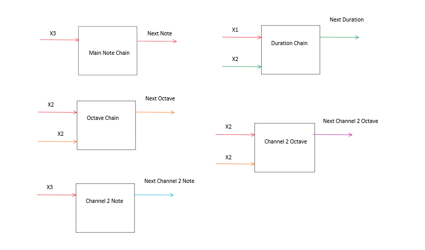
Below is a chart of state dependency. The colors of the arrows indicate the state of the system used/generated in each calculation, while each text represents the order of the state in that dimension. As seen below, the Main Note chain is dependent on the Previous three notes. We additionally have a duration chain which is dependent on the previous note and two previous durations. The Octave chain is used to determine the output note’s octave, The chosen output note is Next Note + Next Octave * 12 because there are 12 half-steps in one octave. By Making the structure of concurrently synthesized notes the same, the main transition matrices could be reused, further conserving memory. Altogether, the transition matrices require about 36K of memory.
Figure 4: Markov chain Diagram
We believe that there is a fair amount of experimentation to be done regarding the structure of the sub-chains in relation to the main chain to maximize output song quality. It is also unknown whether this method of markov sub-chains results in a higher sound quality versus a single transition matrix that includes all of these elements.
Additive Synthesis is a form of synthesis that allows multiple sounds to be played on the same channel. We wanted to make use of Additive synthesis in our final designs because it allows for the generated music to have more depth in its output. Having a two channel output allows for the PIC-32 to play chords and even base resembling the training data. Additive synthesis, along with the paradigm of concurrent note probability processing (as described in the section titled “Concurrent Note Probability”), allows for distinct baselines to be heard in the resulting music. This phenomenon could clearly be heard in the first musical demo shown below in the section titled
This simply entails adding frequencies as the DAC output is assigned. Thus, multiple accumulator variables were included so three differential equations and channels of FM synthesis equations could be computed simultaneously. We then divided the magnitude of each channel by 3 and added them as they entered the DAC.
This, in conjunction with additional Markov chain states, allowed for the simultaneous synthesis of notes on the output of the chain.
Our Algorithm works by first starting in a predetermined state by the user. They must set the previous notes, octaves, and note durations for the algorithm to start at a state with nonzero transition probabilities.
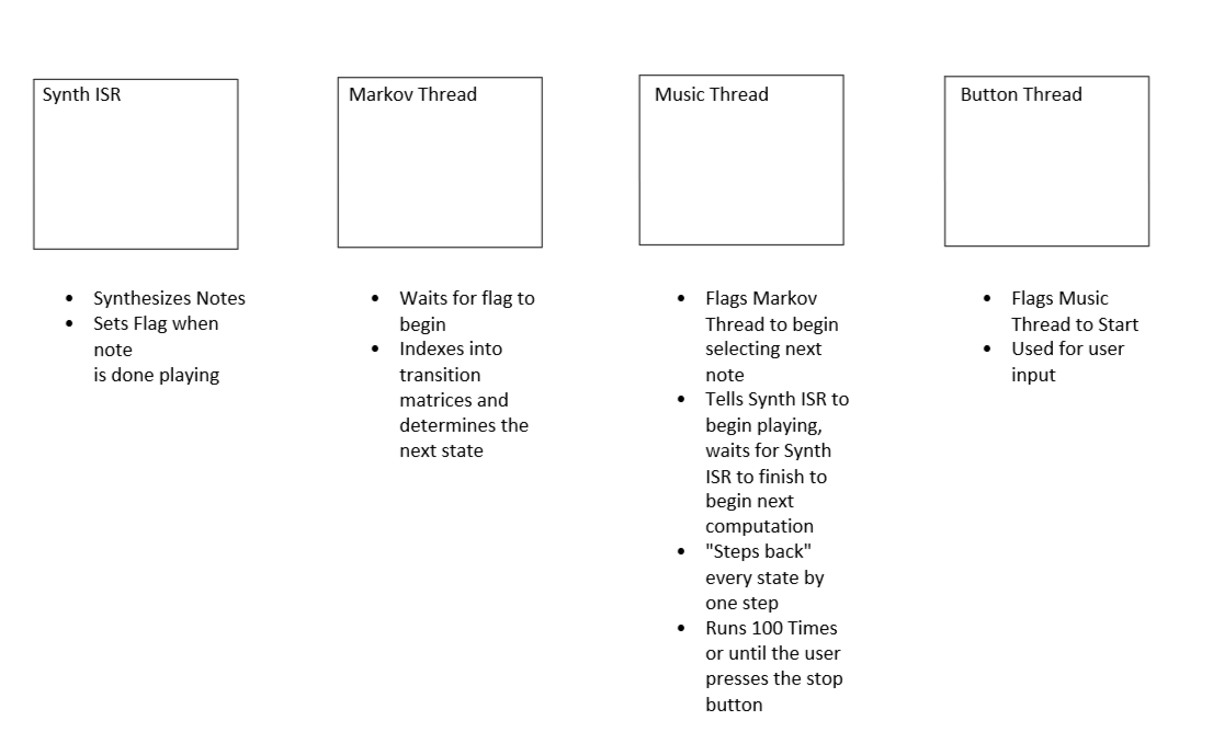
The algorithm is distributed between four different threads. The diagram below shows their jobs when running the algorithm.
Figure 5: Threads Responsible for Markov chain Operation
The Markov Thread is the core of our algorithm, as it determines the next note to be played by the system. This thread waits for a flag from the Music Thread, at this point it indexes into every transition matrix using the current states and then iterates through each matrix using a for loop. After selecting the next state, it is stored in a global variable and then used by the Music Thread.
In each “row” of the Markov chain with next state probabilities we treat each bucket as the probability mass function. This cumulative probability of every index in the row must be equal to 255 (max int value of a 1-byte unsigned char). Thus determining the next state requires no complicated mathematics. We simply generate a random number 0 through 255 and check what the next state is using a for loop by iterating through the row and accumulating the probability mass.
The music thread is triggered whenever the duration is complete. Here, this thread will run (if the play button has been hit and the stop button has not) for 100 notes, update the duration, note and octave state variables to the next state, and generate the next set of frequencies by changing the phase increments. It will assert the markov_trigger flag to run the markov algorithm for the next note. Once our ISR determines that there have been the same amount of cycles elapsed as the duration specified, the flag will be asserted to trigger the music thread to advance to its next state ( the next note). Here, duration is defined by the different type of notes and how much of a beat (set by the tempo of 120 beats per minute) it corresponds to. For example, the durations allowed are sixteenth notes, eighth notes, dotted eighth notes, quarter notes, half notes, dotted half notes, and whole notes, which correspond to 0.25, 0.5, 0.75, 1, 1.5, 2, 3, and 4 beats. Since the ISR fires 20 times every millisecond, the beats per minute of 120 corresponds to ten thousand iterations of the ISR. Thus a sixteenth note will be marked as complete after 2.5 thousand iterations of the ISR.
Once our python script generates our transition matrices, we copy and paste these generated values into a header file. We have created a header file for duration, notes, and octave transition matrices. This kept our code neater as these matrices were sometimes over a thousand lines of code. We additionally had a header file to make it easier to switch between different seeds. Any starting set of states for the notes, octaves and durations for the current, previous, and even further back (we called these “previous previous”) states were considered seeds since they were our initial conditions which influenced the next notes to be played. We created a two dimensional structure to ensure that when the user specifies the seed we can use it to index into the right set of octave, note, and duration matrices. In our current implementation, we currently only change the seeds of our note matrices. However, our duration and octave matrices are dependent on the note states as well, so they indirectly get affected.
Python Training Code
From a high level, the main objective of the Python code was to take as input all the training Midi files, process them in order to extract what notes were played and for how long and then to finally populate the three primary Markov chains (note, duration and octave) accordingly such that the PIC could play notes probabilistically using the cumulative probability technique mentioned above
Formatting Input Midi Files
The first step in working with the Midi files was to convert them into a format that could be manipulated using conventional data analysis libraries. We were fortunate enough to chance upon the py_midicsv that we used to convert each Midi file into a CSV. The converted csv can be seen below.
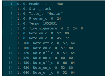
Figure 6: A raw midi file converted to CSV
Essentially, the second column holds the timestamp of the corresponding note switching on or off. The fifth column signifies the note itself while the last column holds the velocity. It was interesting to note that for some notes, column three explicitly mentioned Note_off_c whereas for others, a Note_on_c along with the velocity value going to zero signalled the note turning off. This was an interesting edge case we had to handle in our code.
Another important factor to consider was that the timestamps didn’t really mean anything in absolute values. The sixth column in row one held the clock ticks per beat. That means that each note on duration had to be divided by the ticks per beat to attain the note type (half note, full note etc). The lowest duration went to an eighth of a note (0.125) while the longest duration was a full note (1). Everything in between were multiples of the eighth note up to the full note.
Pre_Processed.csv
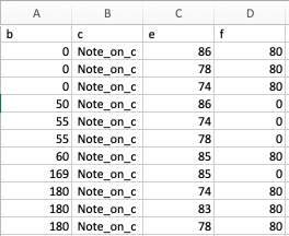
The first step in processing the data was to come up with a new csv that held only those parts of the converted csv that mattered to us. By cleaning out the header and extracting the ticks per beat, we arrived at a cleaned up version of the Midi file which we store in a csv called pre_processed.csv. As one can see, column 1 stores the timestamp (not yet processed into note type), column 2 stores note_on_c or note_off_c, column 3 contains the note Midi number and column 4 contains the velocity value. As mentioned before, with some Midi files, note_off_c was not mentioned explicitly and hence we had to watch out for the velocity going to zero as the note_off signal.
Figure 7: An example of pre_processed.csv
Processed_data.csv
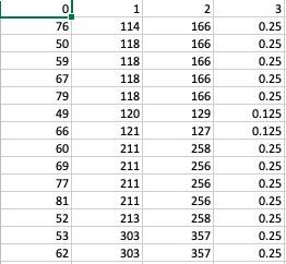
Once we had our data cleaned up and formatted like above, we processed it further such that all the notes were sequentially ordered along with their start and end times. By having their start and end times, we were able to discern the durations. By dividing each duration with the ticks per beat, we were able to obtain the note type for each of those notes. The logic to process processed_data.csv is in lines 73 to 113 in the python file. On closer inspection, one realizes that there is some more arithmetic being done to massage the data to look like below. Part of the reason for the code between 101 and 113 is that not all durations/(ticks_per_beat) were a multiple of 0.125. But as mentioned previously, the duration markov accommodated only 8 distinct note_types and hence all note_types needed to be rounded off to the nearest multiple of 0.125. After some simple arithmetic, we ended up with the following processed_data.
Figure 8: An example of processed_data.csv
Populating the Markov chains
Once we had our processed_data array that looked like the above, it was just a matter of populating the Markov chains appropriately and then copying the transition matrices over to the PIC. As can be seen from lines 120 to 247, we first determined all the notes, durations and the octaves (which were note dependent) that were turned on or off together. Thus the curr_note, curr_duration and curr_octave arrays would hold single or potentially multiple values depending on the Midi file.
Then for the first few iterations of the loop over the processed_data array, the note pipeline (prev_note, prev_x2_note, prev_x3_note) would not be full, i.e. prev_x3_note would be None. In that case, the logic would not populate the Markov chains because the note Markov chain is third order and thus we need three ‘past’ and a current note to index into the 12x12x12x12 note Markov chain.
Once this chain of notes fills up, i.e. each of the previous note arrays have a single or multiple notes, we enter the main loop on line 160. This loop goes through all the notes in all the previous note states (prev, prev_x2, prev_x3 and curr) and bumps up the value at a specific index in the note arkov chain. It is important to note that by subtracting 48 which is the Midi number of the lowest of our 12 notes, we are able to convert all notes to index values from 0 to 12. Thus, each four note combination corresponds to a particular index value in our 12x12x12x12 note Markov chain.
Since the octave Markov only depends on the past two notes, we update its transition matrix only after the prev_x3_note and curr_note loops are finished. We perform similar operations for the duration Markov chain and subsequently update its transition matrix.
Normalizing Probabilities
Once our transition matrices were populated, for each of the last rows of the matrices, i.e. each three note combination in the note Markov chain, each two note, two octave combination in the octave Markov chain and each single note, two duration combination in the duration Markov chain, we added up all the values of the particular row. We then went on to normalize all the elements of that row by dividing them with that cumulative value. Finally, we multiplied all these elements with 255.
This was done for two primary reasons. Firstly, on the PIC side, the way we introduce randomness and select the note to be played is that we generate a random number between 0 and 255 and then iterate through that last row which holds all the normalized values (normalized to 255). Upon iteration, we keep adding up all the normalized values up until the addition of all these normalization values exceed the random number we generated. In this fashion we are able to use cumulative probabilities since a combination is more likely to be played when it has occurred more in the training phase. An oft occurring sequence would have a higher normalized value and hence a higher chance to be the stopping point at which the cumulative probability exceeds the random number. Secondly, we chose the number 255 because we wanted to be space efficient and all numbers upto 255 can be represented by a char which is only a single byte as compared to the four bytes of an integer.
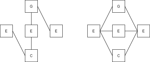
In earlier versions of the system, probability state chaining worked as in Figure 8. Naively, if notes were played at the same time the system would view their states as a series chain. This would cause the algorithm to play arpeggios more frequently, because notes are played concurrently in many songs.
The final algorithm for creating Markov chains creates transition matrix probabilities using the paradigm on the right of Figure 8. A for loop is used to count a state for each possible state involving notes that start at the same time. This makes it so the resulting Markov chain does not have states in a single line. This means that for synthesizing multiple notes at the same time, the resulting synthesis could play chords present in the song.
Figure 8: Diagram of How State Transitions are Added To System (read from left to right)
For the synthesis of multiple notes concurrently we made additional notes dependent on the previous three played notes. This is because we wanted to keep with the paradigm that the main note chain “steers” the song, while the others just follow it. Additional notes played could reuse the octave and note transition matrices.
To actually synthesize the notes, we copied over state variables and had the ISR perform identical calculations with different frequencies as inputs to the system. At the writing of bits to the ISR, we would add together the outputs of individual FM synthesis calculations.
We experimented with up to three notes being played concurrently, but determined the output sounded poor. This is because there is always a chance of dissonant notes being played, and having three tones played concurrently increases this probability. Therefore, we decreased the amount of synthesis channels to two.
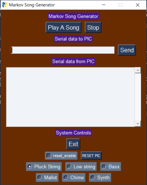
We made some modifications to the standard 4760 GUI to change up the color scheme and match the theme of our project as a music generator. This color scheme change was done by changing the background color and the heading color. We also added “Play A Song” and a “Stop” buttons to play and stop music accordingly, as well as radio buttons to change instruments.
Figure 9: Screenshot of Python GUI
To implement the play and stop buttons, we implemented a button thread that would yield until a new_button flag was asserted, indicating the button was pressed. This would then clear the new_button flag. If the play button was asserted, it would assert the play_music flag, allowing the music thread to operate, and resetting the beat count, note count and tempo flags to ensure it is reset for the music it is about to play. If the stop button is pressed, the play_music flag is cleared and the music thread can no longer run.
A radio thread was implemented to select different instruments. Here, a series of if statements were run to select the corresponding envelopes and tonal quality of the instruments based on the radio button selected. For example, the first radio button selected a pluck string instrument.
A command thread was used to get string user input from the GUI. Here, the input buffer was indexed and the first two characters determined the command, “cs” for change seed, and “ct” for change tempo. The third and fourth characters determined the value being sent, which was casted to an int. For changing the tempo, this value set current tempo directly. To change seeds, this value was the index for the note_seeds 2-Dimensional array for the initial states.
We benchmarked success as the ability to generate music that produced sounds that were pleasant to listen to and not dissonant tones. With single tones generated sequentially, we considered this to be successful as the music was not dissonant, being trained well by the training data. This stayed true after additive synthesis and we noticed our notes sounding well together even in chords of two notes. However, we opted to not use three notes in the system as when we tested three note chords, it began to sound very dissonant. Thus, we consider our two note additive synthesis implementation a success.
One could argue that the music we generated only sounds musical through bias and looking for patterns, even when it may not be there. It could be argued that the music generated is random and a random “musical” pattern can sometimes be generated. While these questions are justified, our algorithm proves more robust than this since it has been shown to generate music with patterns for different seeds tested. Additionally, the music sounds more cohesive on a single song training data rather than multiple songs of different keys and styles within ragtime music. This adds to the argument that these patterns are learned from the data as one could argue that this large multiple songs data set is closer to random than a single song, and the results show this as well.
The goal of this project was to generate music with patterns and cadences to sound “musical” without sounding random and dissonant. Given the variation of cadence and intervals in our music generated and the surprise it elicits every time it is run, we believe that this is a success. The music has been pleasant to the ear and is fascinating to listen to. We believe that there are a wide range of avenues to explore here to take this project even further and believe it is exciting to see what could happen if this is extended to larger order chains through either further memory optimization or external memory units.
The code we reused came from Bruce’s example code for FM synthesis. Our python code used the Numpy, Pandas, OS, and py_midicsv libraries. Since this implementation to generate music with Markov chains is new for the PIC-32, there are opportunities to publish this novel work.
Markov chain Music Generation is a relatively niche topic, with not much documentation or research done on it. The only other instances of its existence are within a couple of YouTube videos. Below are some desired future improvements we thought of over the course of development on this project.
One improvement we believe would greatly improve this project is nearest-neighbor probability matching. This is a modification of our concurrent probability algorithm. It makes more sense to map the probabilities of notes to their nearest one or two neighbors on the scale. This would allow for distinct baselines to be created in the output song.
Figure 9: Diagram of Sample Nearest-Neighbor Note Matching
This improvement is less-elegant than the others, but this would be a simple solution to improving the sound of the resulting Markov chain. Having more memory on the device would allow us to increase transition matrix complexity and thus (potentially) create better sounding music.
Being able to copy training data at runtime on the PIC-32 would allow for an increased degree of user-friendliness. This would require a large amount of manual flash memory manipulation, but if successful this could be packaged into a consumer product of some sort. Users would be able to use their own midi training data and upload it to the PIC-32 without having to compile transition matrices onto the device like we have been doing. This would also allow us to place the PIC in a museum or other exhibit.
The group approves this report for inclusion on the course website.
The group approves the video for inclusion on the course youtube channel.
William: Worked on the overall Markov algorithm, created the optimization to separate notes into notes and octave Markov chains, worked on additive synthesis on the PIC-32.
Rishi: Worked on PIC-32 to implement the music thread as well as respond to the GUI inputs for different instruments, seeds, and play/stop buttons. Also worked on the python GUI itself.
Raghav: Worked on the Python script for training based on the midi files of songs imported.
Protothread Library
https://people.ece.cornell.edu/land/courses/ece4760/PIC32/index_sound_synth.html
https://en.wikipedia.org/wiki/Frequency_modulation_synthesis
https://www.youtube.com/watch?v=K866IyvIAA8&t=105s&ab_channel=AaronVanzylAaronVanzyl
Algorithmic Composition (junshern.github.io)
/*********************************************************************
*
* FM synth to SPI to MCP4822 dual channel 12-bit DAC
*
*********************************************************************
* Bruce Land Cornell University
* Sept 2018
*~~~~~~~~~~~~~~~~~~~~~~~~~~~~~~~~~~~~~~~~~~~~~~~~~~~~~~~~~~~~~~~~~~~~
*/
////////////////////////////////////
// clock AND protoThreads configure!
// You MUST check this file!
#include "config_1_3_2.h"
// threading library
#include "pt_cornell_1_3_2_python.h"
// for sine
#include <math.h>
////////////////////////////////////
// graphics libraries
// SPI channel 1 connections to TFT
#include "tft_master.h"
#include "tft_gfx.h"
// need for rand function
#include <stdlib.h>
// need for sin function
#include <math.h>
#include "Notes.h"
#include "note_markov.h"
#include "duration_markov.h"
#include "octave_markov.h"
#include "markov_seeds.h"
////////////////////////////////////
// === thread structures ============================================
// thread control structs
// note that UART input and output are threads
static struct pt pt_cmd, pt_tick;
// uart control threads
static struct pt pt_input, pt_output, pt_DMA_output ;
// system 1 second interval tick
int sys_time_seconds ;
// === GCC s16.15 format ===============================================
#define float2Accum(a) ((_Accum)(a))
#define Accum2float(a) ((float)(a))
#define int2Accum(a) ((_Accum)(a))
#define Accum2int(a) ((int)(a))
// the native type is _Accum but that is ugly
typedef _Accum fixAccum ;
#define onefixAccum int2Accum(1)
//#define sustain_constant float2Accum(256.0/20000.0) ; // seconds per decay update
// === GCC 0.16 format ===============================================
#define float2Fract(a) ((_Fract)(a))
#define Fract2float(a) ((float)(a))
// the native type is _Accum but that is ugly
typedef _Fract fixFract ;
fixFract onefixFract = float2Fract(0.9999);
// ???
///#define sustain_constant float2Accum(256.0/20000.0) ; // seconds per decay update
/* ====== MCP4822 control word =========================================
bit 15 A/B: DACA or DACB Selection bit
1 = Write to DACB
0 = Write to DACA
bit 14 ? Don?t Care
bit 13 GA: Output Gain Selection bit
1 = 1x (VOUT = VREF * D/4096)
0 = 2x (VOUT = 2 * VREF * D/4096), where internal VREF = 2.048V.
bit 12 SHDN: Output Shutdown Control bit
1 = Active mode operation. VOUT is available. ?
0 = Shutdown the selected DAC channel. Analog output is not available at the channel that was shut down.
VOUT pin is connected to 500 k???typical)?
bit 11-0 D11:D0: DAC Input Data bits. Bit x is ignored.
*/
// A-channel, 1x, active
#define DAC_config_chan_A 0b0011000000000000
#define DAC_config_chan_B 0b1011000000000000
#define Fs 20000.0
#define two32 4294967296.0 // 2^32
//== Timer 2 interrupt handler ===========================================
// actual scaled DAC
volatile unsigned int DAC_data;
// SPI
volatile SpiChannel spiChn = SPI_CHANNEL2 ; // the SPI channel to use
volatile int spiClkDiv = 2 ; // 20 MHz max speed for this DAC
// the DDS units: 1=FM, 2=main frequency
volatile unsigned int phase_accum_fm, phase_incr_fm ;//
volatile unsigned int phase_accum_main, phase_incr_main ;//
// DDS sine table
#define sine_table_size 256
volatile fixAccum sine_table[sine_table_size];
// envelope: FM and main frequency
volatile fixAccum env_fm, wave_fm, dk_state_fm, attack_state_fm;
volatile fixAccum env_main, wave_main, dk_state_main, attack_state_main;
volatile unsigned int phase_accum_fma, phase_incr_fma ;//
volatile unsigned int phase_accum_maina, phase_incr_maina ;//
volatile fixAccum env_fma, wave_fma, dk_state_fma, attack_state_fma;
volatile fixAccum env_maina, wave_maina, dk_state_maina, attack_state_maina;
// define the envelopes and tonal quality of the instruments
#define n_synth 8
// 0 plucked string-like
// 1 slow rise
// 2 string-like lower pitch
// 3 low drum
// 4 medium drum
// 5 snare
// 6 chime
// 7 low, harsh string
//nc - below are various parameters that are used to generate instrument like sounds. They are used in
//in the ISR where sound is produced via the ADC.
// 0 1 2 3 4 5 6 7
volatile fixAccum attack_main[n_synth] = {0.001, 0.9, 0.001, 0.001, 0.001, 0.001, 0.001, .005};
volatile fixAccum decay_main[n_synth] = {0.98, 0.97, 0.98, 0.98, 0.98, 0.80, 0.98, 0.98};
//
volatile fixAccum depth_fm[n_synth] = {2.00, 2.5, 2.0, 3.0, 1.5, 10.0, 1.0, 2.0};
volatile fixAccum attack_fm[n_synth] = {0.001, 0.9, 0.001, 0.001, 0.001, 0.001, 0.001, 0.005};
volatile fixAccum decay_fm[n_synth] = {0.80, 0.8, 0.80, 0.90, 0.90, 0.80, 0.98, 0.98};
//nc - Generating sound is same as in lab 1, however this time we modulate the main frequency (freq_main)
//with another frequency (freq_fm). This is known as frequency modulation.
// 0 1 2 3 4 5 6 7
float freq_main[n_synth] = {1.0, 1.0, 0.5, 0.25, 0.5, 1.00, 1.0, 0.25};
float freq_fm[n_synth] = {3.0, 1.1, 1.5, 0.4, 0.8, 1.00, 1.34, 0.37};
// the current setting for instrument (index into above arrays)
//nc - The current instrument is set to a plucked string.
int current_v1_synth=0, current_v2_synth=0 ;
//20 counts / 1 ms * 1000 msec / 1sec * 60 sec /1 min * min/beats= ( 1.2*10^6)/bpm
#define BPM_SCALER 1200000
#define BPM 120
//nc - When indexing note array - subtract from MIDI number of the first note of the array!
//For ex if C4 is first then subtract by 60. This is done, so that the code can index into the note
//array just on the basis of a midi number.
//nc - tempo is how long the note lasts. The ADC fires at the same rate always, but temp decides how many
//times the ADC produces sounds.(250ms is 5000 ISR fires. Everytime the iSR fires, it produces sound.)
// note transition rate in ticks of the ISR
// rate is 20/mSec (timer overflow rate for the ISR). So 250 mS is 5000 counts
//20 counts (ISR fires) per ms
// 8/sec, 4/sec, 2/sec, 1/sec (4th of sec = 250ms = 5000 counts)
//1 in the sub_divs is a quarter-note
//This array is analagous to note duration
//16th, 8th, dotted_8th, quarter, dotted_quarter, half, dotted half, whole
#define note_dimension 12
_Accum sub_divs[8] = {0.25, 0.5, 0.75, 1, 1.5, 2, 3, 4};
int tempo_v1_flag, tempo_v2_flag;
int current_v1_tempo=1, current_v2_tempo=2;
int tempo_v1_count, tempo_v2_count;
unsigned int cycles_per_beat = BPM_SCALER/BPM;
//MARKOV CHAIN - DURATION
//matrix of probabilities, each row needs to sum up to 1
//can store markov_duration in RAM since (8^4 = 4096 bytes) and RAM is 32K bytes
//Flash memory is 128K bytes but approximating ~28K bytes for the code, we have ~100K bytes for the
//note markov chain. Hence, we could have 17^4 = 83.5K bytes
#define MARKOVDIM 12
//seeds for the markov chains
volatile int prev_prev_note = 11;//rightmost
volatile int prev_note = 11; //center
volatile int curr_note = 3;//leftmost
volatile int next_note = 0;
volatile int prev_prev_note_duration = 0; //rightmost
volatile int prev_note_duration = 0; //middle of tuple
volatile int curr_note_duration = 7; //leftmost of tuple
volatile int next_note_duration = 1; // next note predicted by algo
volatile int prev_octave = 0;
volatile int curr_octave = 0;
volatile int next_octave =0;
//for additive synthesis (chords)
volatile int curr_notea = 3;
volatile int next_notea = 0;
volatile int curr_octavea = 2;
volatile int next_octavea =0;
volatile char seed = 0;
char markov_trigger = 1; //trigger markov thread
// beat/rest patterns
#define n_beats 11
int beat[n_beats] = {
0b0101010101010101, // 1-on 1-off phase 2
0b1111111011111110, // 7-on 1-off
0b1110111011101110, // 3-on 1-off
0b1100110011001100, // 2-on 2-off phase 1
0b1010101010101010, // 1-on 1-off phase 1
0b1111000011110000, // 4-on 4-off phase 1
0b1100000011000000, // 2-on 6-off
0b0011001100110011, // 2-on 2-off phase 2
0b1110110011101100, // 3-on 1-off 2-on 2-off 3-on 1-off 2-on 2-off
0b0000111100001111, // 4-on 4-off phase 2
0b1111111111111111 // on
} ;
// max-beats <= 16 the length of the beat vector in bits
#define max_beats 16
int current_v1_beat=1, current_v2_beat=2;
int beat_v1_count, beat_v2_count ;
//
// random number
int rand_raw ;
// time scaling for decay calculation
volatile int dk_interval; // wait some samples between decay calcs
// play flag
//When this flag is a 1, the ADC plays the note. If the user inputs cs, then the cmd thread
//will flip this flag to a 1
volatile int play_trigger;
volatile fixAccum sustain_state, sustain_interval=0;
// profiling of ISR
volatile int isr_time, isr_start_time, isr_count=0;
volatile int flag_attack_done = 0;
volatile int cycles_attack = 0;
// === outputs from python handler =============================================
// signals from the python handler thread to other threads
// These will be used with the prototreads PT_YIELD_UNTIL(pt, condition);
// to act as semaphores to the processing threads
char new_string = 0;
char new_button = 0;
char new_toggle = 0;
char new_slider = 0;
char new_list = 0 ;
char new_radio = 0 ;
char play_music = 0;
char note_count = 0; // max 255
// identifiers and values of controls
// curent button
char button_id, button_value ;
// current toggle switch/ check box
char toggle_id, toggle_value ;
// current radio-group ID and button-member ID
char radio_group_id, radio_member_id ;
// current slider
int slider_id;
float slider_value ; // value could be large
// current listbox
int list_id, list_value ;
// current string
char receive_string[64];
//=============================
void __ISR(_TIMER_2_VECTOR, ipl2) Timer2Handler(void)
{
// time to get into ISR
isr_start_time = ReadTimer2();
tempo_v1_count++ ;
// update flag if duration specified was hit
if (tempo_v1_count>=cycles_per_beat*sub_divs[curr_note_duration]) {
tempo_v1_flag = 1;
tempo_v1_count = 0;
}
mT2ClearIntFlag();
//Everytime the timer interrupts, the phase_accum variable for both the main_freq and freq_mod
//vector increments. This is irrespective of sound being played or not.
// FM phase
phase_accum_fm += phase_incr_fm ;
// main phase
phase_accum_main += phase_incr_main + (Accum2int(sine_table[phase_accum_fm>>24] * env_fm)<<16) ;
phase_accum_fma += phase_incr_fma ;
// main phase
phase_accum_maina += phase_incr_maina + (Accum2int(sine_table[phase_accum_fma>>24] * env_fma)<<16) ;
// init the exponential decays
// by adding energy to the exponential filters
if (play_trigger) {
//nc - current_v1_synth contains the index of the instrument to be played.
//hence all appropriate variables required to produce that instrument's sound are
//extracted below.
dk_state_fm = depth_fm[current_v1_synth];
dk_state_main = onefixAccum;
dk_state_fma = depth_fm[current_v1_synth];
dk_state_maina = onefixAccum;
attack_state_fm = depth_fm[current_v1_synth];
attack_state_main = onefixAccum;
attack_state_fma = depth_fm[current_v1_synth];
attack_state_maina = onefixAccum;
play_trigger = 0;
phase_accum_fm = 0;
phase_accum_main = 0;
phase_accum_fma = 0;
phase_accum_maina = 0;
dk_interval = 0;
sustain_state = 0;
flag_attack_done = 0;
}
//Bread and butter of the algorithm
//To note, the following code block runs, even if play_trigger is not set.
//Main frequency and modulating frequency are BOTH present
//pure tone with the modulator decaying
//in guitar string the second harmonic decays faster than the fundamental, and third even faster
// envelope calculations are 256 times slower than sample rate
// computes 4 exponential decays and builds the product envelopes
if ((dk_interval++ & 0xff) == 0){
// approximate the first order FM decay ODE
dk_state_fm = dk_state_fm * decay_fm[current_v1_synth] ;
// approximate the first order main waveform decay ODE
dk_state_main = dk_state_main * decay_main[current_v1_synth] ;
dk_state_fma = dk_state_fma * decay_fm[current_v1_synth] ;
// approximate the first order main waveform decay ODE
dk_state_maina = dk_state_maina * decay_main[current_v1_synth] ;
//}
// approximate the ODE for the exponential rise FM/main waveform
attack_state_fm = attack_state_fm * attack_fm[current_v1_synth];
attack_state_main = attack_state_main * attack_main[current_v1_synth];
attack_state_fma = attack_state_fma * attack_fm[current_v1_synth];
attack_state_maina = attack_state_maina * attack_main[current_v1_synth];
// product of rise and fall is the FM envelope
// fm_depth is the current value of the function
env_fm = (depth_fm[current_v1_synth] - attack_state_fm) * dk_state_fm ;
env_fma = (depth_fm[current_v1_synth] - attack_state_fma) * dk_state_fma ;
// product of rise and fall is the main envelope
env_main = (onefixAccum - attack_state_main) * dk_state_main ;
env_maina = (onefixAccum - attack_state_maina) * dk_state_maina ;
}
//send a value to the DAC irrespective of play trigger being set or not.
// === Channel A =============
// CS low to start transaction
mPORTBClearBits(BIT_4); // start transaction
// write to spi2
WriteSPI2(DAC_data);
//update sinewave values to be sent to the DAC
wave_main = sine_table[phase_accum_main>>24] * env_main;
//second sinewave->to layer as a chord
wave_maina = sine_table[phase_accum_maina>>24] * env_maina;
// truncate to 12 bits, read table, convert to int and add offset
DAC_data = DAC_config_chan_A | ((int)(Accum2int(wave_main)*0.33) + (int)(Accum2int(wave_maina)*0.33) + 2048) ; //change to 0.25 when 4 notes
// test for done
while (SPI2STATbits.SPIBUSY); // wait for end of transaction
// CS high
mPORTBSetBits(BIT_4); // end transaction
// time to get into ISR is the same as the time to get out so add it again
isr_time = max(isr_time, ReadTimer2()+isr_start_time) ; // - isr_time;
} // end ISR TIMER2
// === Serial Thread ======================================================
// revised commands:
// cs note (00-99) -- change seed value (single digit numbers must start with 0, ex. 08)
// t -- print current instrument parameters
//
//nc - This is the main control thread of the program
static PT_THREAD (protothread_cmd(struct pt *pt))
{
// The serial interface
static int value = 0;
static float f_fm, f_main;
PT_BEGIN(pt);
// clear port used by thread 4
mPORTBClearBits(BIT_0);
while(1) {
rand_raw = rand();
//Yield until a new string is received.
PT_YIELD_UNTIL(pt, new_string==1);
new_string = 0;
//nc - value is note index in our own note array in the header
value = (int) (receive_string[2] - '0') * 10 + (receive_string[3] - '0');
switch(receive_string[0]){
case 'c': // value is seed index
if (receive_string[1]=='t') {
// value is tempo index 0-3
current_v1_tempo = (int)(value);
}
//change the seed of the markov chain
if (receive_string[1]=='s') { //seed
seed = (int)(value);
prev_prev_note = note_seeds[seed][2];//rightmost Change index of first thing to seed variable
prev_note = note_seeds[seed][1]; //center
curr_note = note_seeds[seed][0];//leftmost
}
break;
}
// never exit while
} // END WHILE(1)
PT_END(pt);
} // thread 3
// === Thread 5 ======================================================
//Markov thread
static PT_THREAD (protothread_markov(struct pt *pt))
{
PT_BEGIN(pt);
while(1) {
// yield until triggered by music thread
PT_YIELD_UNTIL(pt, markov_trigger == 1) ;
markov_trigger = 0;
unsigned long int random_num = rand() % 255; //max 255 random number
unsigned long int cum_prob = 0;
//duration markov thread-set cumulative probabilities
int i;
for (i=0; i<8; i++){
cum_prob += (unsigned long int)
markov_duration[curr_note][curr_note_duration][prev_note_duration][i];
if (cum_prob >= random_num){ //next note duration based on the largest number lower than the random number
next_note_duration = i;
break;
}
}
//reset cumulative probability
cum_prob = 0;
//note markov chain
random_num = rand() % 255; //255 max number
for (i=0; i<13; i++){
cum_prob += (unsigned long int)
markov_notes[curr_note][prev_note][prev_prev_note][i];
if(cum_prob >= random_num){
next_note = i;
break;
}
}
cum_prob = 0;
//note markov chain - second note in the chord
random_num = rand() % 255; //255 max
for (i=0; i<13; i++){
cum_prob += (unsigned long int)
markov_notes[curr_note][prev_note][prev_prev_note][i];
if(cum_prob >= random_num){
next_notea = i;
break;
}
}
cum_prob = 0;
//octave markov chain
random_num = rand() % 255; //255 max
for (i=0; i<4; i++){
cum_prob += (unsigned long int)
markov_octave[curr_note][prev_note][curr_octave][prev_octave][i];
if(cum_prob >= random_num){
next_octave = i;
break;
}
}
cum_prob = 0;
//octave markov chain, second note in the chord
random_num = rand() % 255; //255 max
for (i=0; i<4; i++){
cum_prob += (unsigned long int)
markov_octave[curr_note][prev_note][curr_octave][prev_octave][i];
if(cum_prob >= random_num){
next_octavea = i;
break;
}
}
// NEVER exit while
} // END WHILE(1)
PT_END(pt);
} // thread 4
// === radio thread =========================================================
// process listbox from Python to set instrument to be played
static PT_THREAD (protothread_radio(struct pt *pt))
{
PT_BEGIN(pt);
while(1){
PT_YIELD_UNTIL(pt, new_radio==1);
// clear flag
new_radio = 0;
if (radio_group_id == 1){
if (radio_member_id == 1){
current_v1_synth = (int)(0);
}
if (radio_member_id == 2){
current_v1_synth = (int)(1);
}
if (radio_member_id == 3){
current_v1_synth = (int)(2);
}
//skip instrument 4 and 6
if (radio_member_id == 5){
current_v1_synth = (int)(4);
}
if (radio_member_id == 7){
current_v1_synth = (int)(6);
}
if (radio_member_id == 8){
current_v1_synth = (int)(7);
}
}
} // END WHILE(1)
PT_END(pt);
} // thread radio
// === Music thread ==========================================================
// process buttons from Python to play music
static PT_THREAD (protothread_music(struct pt *pt))
{
PT_BEGIN(pt);
while(1){
PT_YIELD_UNTIL(pt,tempo_v1_flag==1); //yield until current duration has been met
if (play_music && note_count < 100){ //100 note song
//update values one step further into markov chain
prev_prev_note_duration = prev_note_duration;
prev_note_duration = curr_note_duration;
curr_note_duration = next_note_duration;
prev_prev_note = prev_note;
prev_note = curr_note;
curr_note = next_note;
prev_octave = curr_octave;
curr_octave = next_octave;
curr_notea = next_notea;
curr_octavea = next_octavea;
//generate phase increments based on notes and octaves found
phase_incr_fm = freq_fm[current_v1_synth]*notesDEF[curr_note + 12 * curr_octave]*(float)two32/Fs;
phase_incr_main = freq_main[current_v1_synth]*notesDEF[curr_note + 12 * curr_octave]*(float)two32/Fs;
phase_incr_fma = freq_fm[current_v1_synth]*notesDEF[curr_notea + 12 * curr_octavea]*(float)two32/Fs;
phase_incr_maina = freq_main[current_v1_synth]*notesDEF[curr_notea + 12 * curr_octavea]*(float)two32/Fs;
markov_trigger = 1;//trigger markov thread
play_trigger = 1;//play note
tempo_v1_flag = 0;
note_count++;
}
} // END WHILE(1)
PT_END(pt);
} // thread blink
// === Buttons thread ==========================================================
// process buttons from Python to play and stop music
static PT_THREAD (protothread_buttons(struct pt *pt))
{
PT_BEGIN(pt);
while(1){
PT_YIELD_UNTIL(pt, new_button==1);
// clear flag
new_button = 0;
// Button one -- Play
if (button_id==1 && button_value==1) {
play_music = 1;
tempo_v1_count = 0;
tempo_v1_flag = 0;
note_count = 0;
break;
}
// Button 2 -- Stop
if (button_id==2 && button_value==1) {
play_music = 0; //stop
}
} // END WHILE(1)
PT_END(pt);
} // thread blink
// === Python serial thread ====================================================
// you should not need to change this thread UNLESS you add new control types
static PT_THREAD (protothread_serial(struct pt *pt))
{
PT_BEGIN(pt);
static char junk;
//
//
while(1){
// There is no YIELD in this loop because there are
// YIELDS in the spawned threads that determine the
// execution rate while WAITING for machine input
// =============================================
// NOTE!! -- to use serial spawned functions
// you MUST edit config_1_3_2 to
// (1) uncomment the line -- #define use_uart_serial
// (2) SET the baud rate to match the PC terminal
// =============================================
// now wait for machine input from python
// Terminate on the usual <enter key>
PT_terminate_char = '\r' ;
PT_terminate_count = 0 ;
PT_terminate_time = 0 ;
// note that there will NO visual feedback using the following function
PT_SPAWN(pt, &pt_input, PT_GetMachineBuffer(&pt_input) );
// Parse the string from Python
// There can be toggle switch, button, slider, and string events
// pushbutton
if (PT_term_buffer[0]=='b'){
// signal the button thread
new_button = 1;
// subtracting '0' converts ascii to binary for 1 character
button_id = (PT_term_buffer[1] - '0')*10 + (PT_term_buffer[2] - '0');
button_value = PT_term_buffer[3] - '0';
}
// // listbox
if (PT_term_buffer[0]=='l'){
new_list = 1;
list_id = PT_term_buffer[2] - '0' ;
list_value = PT_term_buffer[3] - '0';
}
// radio group
if (PT_term_buffer[0]=='r'){
new_radio = 1;
radio_group_id = PT_term_buffer[2] - '0' ;
radio_member_id = PT_term_buffer[3] - '0';
}
// string from python input line
if (PT_term_buffer[0]=='$'){
// signal parsing thread
new_string = 1;
// output to thread which parses the string
// while striping off the '$'
strcpy(receive_string, PT_term_buffer+1);
}
} // END WHILE(1)
PT_END(pt);
} // thread blink
// === Main ======================================================
// set up UART, timer2, threads
// then schedule them as fast as possible
int main(void)
{
// === config the uart, DMA, vref, timer5 ISR =============
PT_setup();
// === setup system wide interrupts ====================
INTEnableSystemMultiVectoredInt();
// 400 is 100 ksamples/sec
// 1000 is 40 ksamples/sec
// 2000 is 20 ksamp/sec
// 1000 is 40 ksample/sec
// 2000 is 20 ks/sec
OpenTimer2(T2_ON | T2_SOURCE_INT | T2_PS_1_1, 2000);
// set up the timer interrupt with a priority of 2
ConfigIntTimer2(T2_INT_ON | T2_INT_PRIOR_2);
mT2ClearIntFlag(); // and clear the interrupt flag
// SCK2 is pin 26
// SDO2 (MOSI) is in PPS output group 2, could be connected to RB5 which is pin 14
PPSOutput(2, RPB5, SDO2);
// control CS for DAC
mPORTBSetPinsDigitalOut(BIT_4);
mPORTBSetBits(BIT_4);
// divide Fpb by 2, configure the I/O ports. Not using SS in this example
// 16 bit transfer CKP=1 CKE=1
// possibles SPI_OPEN_CKP_HIGH; SPI_OPEN_SMP_END; SPI_OPEN_CKE_REV
// For any given peripherial, you will need to match these
SpiChnOpen(spiChn, SPI_OPEN_ON | SPI_OPEN_MODE16 | SPI_OPEN_MSTEN | SPI_OPEN_CKE_REV , spiClkDiv);
// === now the threads ====================
// init the display
tft_init_hw();
tft_begin();
tft_fillScreen(ILI9340_BLACK);
//240x320 vertical display
tft_setRotation(1); // Use tft_setRotation(1) for 320x240
// === identify the threads to the scheduler =====
// add the thread function pointers to be scheduled
// --- Two parameters: function_name and rate. ---
// rate=0 fastest, rate=1 half, rate=2 quarter, rate=3 eighth, rate=4 sixteenth,
// rate=5 or greater DISABLE thread!
prev_prev_note = note_seeds[seed][2];//rightmost Change index of first thing to seed variable
prev_note = note_seeds[seed][1]; //center
curr_note = note_seeds[seed][0];//leftmost
prev_prev_note_duration = duration_seeds[seed][2]; //rightmost
prev_note_duration = duration_seeds[seed][1]; //middle of tuple
curr_note_duration = duration_seeds[seed][0]; //leftmost of tuple
prev_octave = octave_seeds[seed][1];
curr_octave = octave_seeds[seed][0];
pt_add(protothread_cmd, 0);
pt_add(protothread_serial, 0);
pt_add(protothread_markov, 0);
pt_add(protothread_buttons, 0);
pt_add(protothread_music,0);
pt_add(protothread_radio,0);
// === initalize the scheduler ====================
PT_INIT(&pt_sched) ;
// >>> CHOOSE the scheduler method: <<<
// (1)
// SCHED_ROUND_ROBIN just cycles thru all defined threads
//pt_sched_method = SCHED_ROUND_ROBIN ;
// NOTE the controller must run in SCHED_ROUND_ROBIN mode
// ALSO note that the scheduler is modified to cpy a char
// from uart1 to uart2 for the controller
pt_sched_method = SCHED_ROUND_ROBIN ;
// // init the threads
// PT_INIT(&pt_cmd);
// PT_INIT(&pt_tick);
// turn off the sustain until triggered
sustain_state = float2Accum(100.0);
// build the sine lookup table
// scaled to produce values between 0 and 4095
int k;
for (k = 0; k < sine_table_size; k++){
sine_table[k] = float2Accum(2047.0*sin((float)k*6.283/(float)sine_table_size));
}
// === scheduler thread =======================
// scheduler never exits
PT_SCHEDULE(protothread_sched(&pt_sched));
// ===========================================
} // main
PYTHON CODE
import py_midicsv as pm
import pandas as pd
import os
import numpy as np
#Pathnames for files to be loaded from or saved to
curr_path = os.path.dirname(os.path.abspath(__file__)) #current path
midiFile = os.path.join(curr_path, "test4.mid") #midiFile to be parsed
outFile = os.path.join(curr_path, "output.csv") #Raw CSV from midi file
no_headers_csv = os.path.join(curr_path, "no_headers.csv") #CSV after removing the headers and footers
processed_data_csv = os.path.join(curr_path, "processed_data.csv") #Contains: Note, start time, end time, duration (end time-start time)
markov_note_file = os.path.join(curr_path, "MarkovNote.txt") #Markov chains generated for notes-to be added to header file in PIC32
markov_duration_file = os.path.join(curr_path, "MarkovDuration.txt") #Markov chains generated for duration-to be added to header file in PIC32
markov_octave_file = os.path.join(curr_path, "MarkovOctave.txt") #Markov chains generated for ocatve-to be added to header file in PIC32
seeds_file = os.path.join(curr_path, "Seeds.txt") #Seeds that determine the notes, durations and octaves to start the algorithm from
#create numpy array that is 13x13x13x13 for notes and 8x8x8x8 for duration. All populated by 0s
markov_note = np.full((12,12,12,12),0)
markov_octave = np.full((12,12,4,4,4),0) #n^6 and we have n = 4 octaves (Current octave depends on 3 notes and 2 past octaves)
markov_duration = np.full((12,8,8,8),0)
#Parse midi file and convert to CSV
directory = os.path.join(curr_path, 'training-data')
for filename in os.listdir(directory):
if filename.endswith(".mid") or filename.endswith(".midi"):
midiFile = os.path.join(directory, filename)
# Load the MIDI file and parse it into CSV format
csv_string = pm.midi_to_csv(midiFile)
with open(outFile, "w") as f: #write to output.csv file
f.write("a, b, c, d, e, f\n")
f.writelines(csv_string)
f.close()
endMidi = pd.read_csv(outFile,error_bad_lines=False)
#access the first row and convert to numpy array, to get the ticks per beat
firstRow = endMidi.loc[[0]].to_numpy()
#(Note_off - Note_on)/ ticks_per_beat = note type (1/8th etc)
ticks_per_beat = firstRow[0,5]
if (type(ticks_per_beat) == str):
ticks_per_beat.strip() #remove whitespaces from the string, only store the number. To be converted to float
ticks_per_beat = float(ticks_per_beat)
endMidi.drop(endMidi.columns[[0,3]], axis=1,inplace = True) #remove columns 0 to 3. Modify inplace, not a copy
# .shape returns the dimensions of the dataframe
# Check every row for the first instance of "Note_on_C" to show the start of a note being played. Delete all prior rows
for row_index in range(endMidi.shape[0]):
if (endMidi.iloc[row_index, 1]).strip() == 'Note_on_c':
endMidi = endMidi.iloc[row_index:] #Delete every row before this first instance of note_on_c
break
#check every row from the bottom for the first instance of "Note_off_C" or "Note_on_C"
#Delete every row after it
for row_index in range(endMidi.shape[0] - 1, -1, -1):
if ((endMidi.iloc[row_index, 1].strip() == 'Note_on_c') or (endMidi.iloc[row_index, 1].strip() == 'Note_off_c')):
endMidi = endMidi.iloc[:row_index]
break
#convert this dataframe with removed headers and footers to CSV
endMidi.to_csv(no_headers_csv, index = False)
endMidi = endMidi.to_numpy() #convert to numpy array
processed_data = []
#1 loop through the notes in csv (column 3)
#2 identify unique notes, insert them in 2D array and store the start time (assuming first hit of unique note is always turn on)
#3 as soon as we identify a repeated note, we get the end time, subtract to get duration (assuming second hit of note is always turn off)
# 2D array contains: (notes, start time, end time, duration)
for index in range(endMidi.shape[0]):
on_or_off = endMidi[index, 1] #store on_or_off string value
if (type(on_or_off) == str):
on_or_off = on_or_off.strip() #remove whitespace
#skips over rows that don't contain note_on_c or note_off_c or have notes out of range from our implementation
if ((on_or_off != 'Note_on_c' and on_or_off != 'Note_off_c') or int(endMidi[index][2]) < 24 or int(endMidi[index][2]) > 71):
continue
#get velocity, having a note on with velocity = 0 is equivalent to note_off
velocity = endMidi[index, 3]
if (type(velocity) == str):
velocity = velocity.strip()
velocity = int(velocity)
#if the note is on, add its note value and start tick to 2D array
if (on_or_off == 'Note_on_c') and (velocity != 0):
processed_data.append([endMidi[index, 2], endMidi[index, 0], None, None])
elif ((velocity == 0) and (on_or_off == 'Note_on_c')) or (on_or_off == 'Note_off_c'):
#elif the note is off, start iterating from the bottom of the processed_data (not endMidi)
for index2 in range(len(processed_data) - 1, -1, -1):
#if the endMidi off note (lets say it's 50) is same as the most recently added note (of the same kind, so 50) in processed_data,
#we can be assured that that is an on note
if (endMidi[index, 2] == processed_data[index2][0]):
#hence, save as end time on index2 note of processed_data, the time of the index note in endMidi
processed_data[index2][2] = endMidi[index, 0]
#store duration: note type (quarter note, half note, full note etc )
processed_data[index2][3] = (processed_data[index2][2] - processed_data[index2][1]) / ticks_per_beat
#multiply by 8 because our smallest duration is 0.125 and we want to normalize to 1. Since there are a lot of decimals durations,
#the code below is a way to round them all off to multiples of 0.125.
#so first multiply by 8
processed_data[index2][3] *= 8
#now round to a decimal
processed_data[index2][3] = round(processed_data[index2][3])
if (processed_data[index2][3] == 0): #if the note type is below an eighth, make it an eighth.
processed_data[index2][3] = 1
if (processed_data[index2][3] > 8): #if the note type is longer than a full note, reduce it to a note.
processed_data[index2][3] = 8
processed_data[index2][3] /= 8 #Divide by 8 to bring back to decimal values.
break
processed_data_df = pd.DataFrame(processed_data)
processed_data_df.to_csv(processed_data_csv, index = False)
# savetxt(processed_data_csv, processed_data, delimiter=',')
#instantiate the note, duration and octave pipelines.
curr_note = None
prev_note = None
prev_x2_note = None
prev_x3_note = None
curr_duration = None
prev_duration = None
prev_x2_duration = None
prev_x3_duration = None
curr_octave = None
prev_octave = None
prev_x2_octave = None
#go through each row of the processed_data array
for note_array_index in range(len(processed_data)):
#note down the current time to figure out which notes need to be looked at together
curr_start_time = int(processed_data[note_array_index][1])
#Note Parallel Algo
curr_note = []
curr_duration = []
curr_octave = []
#from the current index in the processed data, iterate down the processed_data array to add notes,
#durations and octaves that all start at the same time
for note_array_index_2 in range(note_array_index,len(processed_data)-note_array_index):
#check if the start time of the note at note_array_index_2 is equal to the start time of the note at note_array_index.
#if not, break.
if(processed_data[note_array_index_2][1] != curr_start_time):
break
#if it is, add note, duration and octave to their respective arrays.
#the octave is essentially a value between 0 and 3 inclusive
#using try-catch block since we saw some errors attributed to 'bad' csv lines.
try:
temp_note = int(processed_data[note_array_index_2][0])
curr_note.append(temp_note)
curr_duration.append(float(processed_data[note_array_index_2][3]))
#this gives the octave of the current note relative to our lowest note
curr_octave.append(int((temp_note - 48)/ 12))
except:
print('in except')
continue
#just propogate the chain. This will update the notes, durations and octaves at every time step.
#the loops below use this information to update the markov transition matrices.
#notes
prev_x3_note = prev_x2_note
prev_x2_note = prev_note
prev_note = curr_note
#duration
prev_x3_duration = prev_x2_duration
prev_x2_duration = prev_duration
prev_duration = curr_duration
#octaves
prev_x2_octave = prev_octave
prev_octave = curr_octave
### THIS LOOP UPDATES THE TRANSITION MATRICES FOR ALL MARKOV CHAINS ###
#if the pipeline of notes is not filled, skip updating the matrices
if (prev_x3_note != None):
#at this point, all the current arrays contain atleast a single element, and potentially more than one element.
#the goal for this note 4D loop is to find all permutations of the past three notes with the current note and update the
#12x12x12x12 matrix for each of the combinations.
for prev_note_index in range(len(prev_note)):
for prev_x2_note_index in range(len(prev_x2_note)):
for prev_x3_note_index in range(len(prev_x3_note)):
for curr_note_index in range(len(curr_note)):
try:
#We subtract by 48 in order to normalize for the lowest note Midi number which is 48. After subtracting from 48 and
#modding with 12, we essentially get an index value for each note. Thus each note is able to correspond to a particular index
#value that we are able to increment.......
curr_markov_index_n = (int(curr_note[curr_note_index] - 48)) % 12
prev_markov_index_n = (int(prev_note[prev_note_index] - 48)) % 12
prev_x2_markov_index_n = (int(prev_x2_note[prev_x2_note_index] - 48)) % 12
prev_x3_markov_index_n = (int(prev_x3_note[prev_x3_note_index] - 48)) % 12
#.....here!
markov_note[prev_markov_index_n, prev_x2_markov_index_n, prev_x3_markov_index_n, curr_markov_index_n] += 1
except:
continue
#since the octaves depend on the past two octaves and the past two notes, we do the same.
#take note that we make sure that the current note and prev_x3_note calculation is done before we udpate the octave
#markov because the octave markov only depends on the prev 2 notes, not prev 3.
for curr_octave_index in range(len(curr_octave)):
for prev_octave_index in range(len(prev_octave)):
for prev_x2_octave_index in range(len(prev_x2_octave)):
#these two lines are essentially the same as the ones we wrote when updating the note markov chain above.
prev_markov_index_n = (int(prev_note[prev_note_index] - 48)) % 12
prev_x2_markov_index_n = (int(prev_x2_note[prev_x2_note_index] - 48)) % 12
curr_octave_n = curr_octave[curr_octave_index]
prev_octave_n = prev_octave[prev_octave_index]
prev_x2_octave_n = prev_x2_octave[prev_x2_octave_index]
markov_octave[prev_markov_index_n, prev_x2_markov_index_n, prev_octave_n, prev_x2_octave_n, curr_octave_n] += 1
#do the same for duration markov as well..
if (prev_x2_duration != None):
for prev_duration_index in range(len(prev_duration)):
for prev_x2_duration_index in range(len(prev_x2_duration)):
for curr_duration_index in range(len(curr_duration)):
for prev_note_index_2 in range(len(prev_note)):
#We haven't been too smart with variable naming here, so excuse that :)
#We subtract by 1 because after dividing by 0.125, if the result is 1, then it should actually index into value 0
#and if the value is a 8 (0.125 * 8 = 1), then the increment should be made at index 8.
curr_markov_index_d = int(curr_duration[curr_duration_index] / 0.125) - 1
prev_markov_index_d = int(prev_duration[prev_duration_index] / 0.125) - 1
prev_x2_markov_index_d = int(prev_x2_duration[prev_x2_duration_index] / 0.125) - 1
prev_markov_index_n_2 = (int(prev_note[prev_note_index_2] - 48)) % 12
markov_duration[prev_markov_index_n_2][prev_markov_index_d][prev_x2_markov_index_d][curr_markov_index_d] += 1
else:
continue
#here we loop through the transition matrices to normalize the values to 255
#we normalize to 255 because numbers upto 255 can be expressed as char that are a single byte vs the four bytes for an int.
#this saves space on the PIC.
note_seeds = []
markov_note_dim = 12
for i in range(markov_note_dim):
for j in range(markov_note_dim):
for k in range(markov_note_dim):
#the accumulator variable for normalization
accumulator = 0
for l in range(markov_note_dim):
accumulator += markov_note[i, j, k, l]
if (accumulator != 0):
print((i,j,k))
#appending the seeds -- the non zero probability points to start our music generation from on the PIC.
note_seeds.append([i,j,k])
for t in range(markov_note_dim):
#once we have the accumulator value, loop through all the elements of the last row and normalize to 255.
markov_note[i, j, k, t] = 255 * markov_note[i, j, k, t]
markov_note[i, j, k, t] = int(markov_note[i, j, k, t] / accumulator)
duration_seeds = []
markov_duration_dim = 8
for i in range(markov_note_dim):
for k in range(markov_duration_dim):
for l in range(markov_duration_dim):
accumulator = 0
for m in range(markov_duration_dim):
accumulator += markov_duration[i, k, l, m]
if (accumulator != 0):
#print('hi')
#print((i,k,l))
duration_seeds.append([k,l])
for t in range(markov_duration_dim):
markov_duration[i, k, l, t] = 255 * markov_duration[i, k, l, t]
markov_duration[i, k, l, t] = int(markov_duration[i, k, l, t] / accumulator)
octave_seeds = []
markov_octave_dim = 4
for i in range(markov_note_dim):
for j in range(markov_note_dim):
for k in range(markov_octave_dim):
for l in range(markov_octave_dim):
accumulator = 0
for m in range(markov_octave_dim):
accumulator += markov_octave[i, j, k, l, m]
if (accumulator != 0):
octave_seeds.append([k,l])
for t in range(markov_octave_dim):
markov_octave[i, j, k, l, t] = 255 * markov_octave[i, j, k, l, t]
markov_octave[i, j, k, l, t] = int(markov_octave[i, j, k, l, t] / accumulator)
f= open(markov_note_file,"w+")
coolString = np.array2string(markov_note,threshold = np.sys.maxsize,separator=',')
x = coolString.replace('[','{')
y = x.replace(']','}')
f.write(y+';')
f.close()
f= open(markov_duration_file,"w+")
coolString = np.array2string(markov_duration,threshold = np.sys.maxsize,separator=',')
x = coolString.replace('[','{')
y = x.replace(']','}')
f.write(y+';')
f.close()
f= open(markov_octave_file,"w+")
coolString = np.array2string(markov_octave,threshold = np.sys.maxsize,separator=',')
x = coolString.replace('[','{')
y = x.replace(']','}')
f.write(y+';')
f.close()
f= open(seeds_file,"w+")
coolString = np.array2string(np.array(note_seeds),threshold = np.sys.maxsize,separator=',')
x = coolString.replace('[','{')
y = x.replace(']','}')
f.write('const unsigned char note_seeds [' + str(len(note_seeds)) + '][3] = \n')
f.write(y+';')
coolString = np.array2string(np.array(duration_seeds),threshold = np.sys.maxsize,separator=',')
x = coolString.replace('[','{')
y = x.replace(']','}')
f.write('\nconst unsigned char duration_seeds [' + str(len(duration_seeds)) + '][2] = \n')
f.write(y+';')
coolString = np.array2string(np.array(octave_seeds),threshold = np.sys.maxsize,separator=',')
x = coolString.replace('[','{')
y = x.replace(']','}')
f.write('\nconst unsigned char octave_seeds [' + str(len(octave_seeds)) + '][2]= \n')
f.write(y+';')
f.close()
processed_data_df = pd.DataFrame(processed_data)
processed_data_df.to_csv(outFile,index = False)