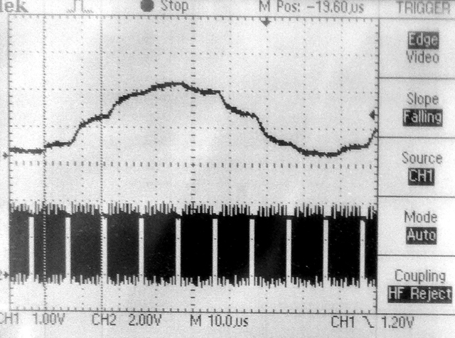
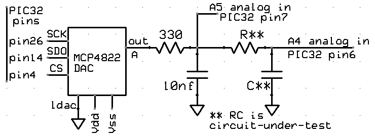
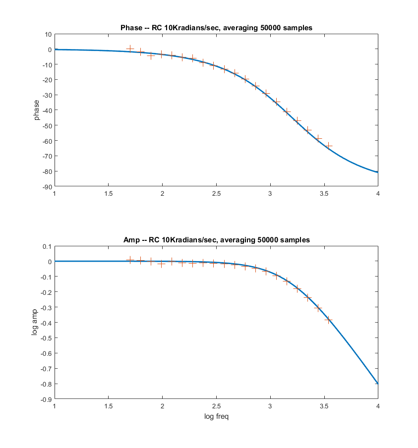
It is useful to get the phase and magnitude of response of a circuit as a function of frequency. A DDS unit is used to synthesize a cosine wave, which is then played through a SPI attached DAC. The output of the DAC is attached to the circuit under test. For starts, I am just testing on an RC lowpass with a nominal cutoff frequency of 10000 radians/sec (1590 Hz) and a resistance of 10 kohm. The voltage across the capacitor feeds back to the AN4 analog input (pin 6). An ISR does the DDS sine synthesis, records the voltage, and computes the quadrature values by multiplying the analog input voltage with the DDS value (I-signal) and a sine wave in quadrature with the DDS value (Q-signal). The quadrature signals, which have zero average frequency (product of two equal frequencies) are lowpass filtered in the ISR, then the main thread computes the phase and magnitude. Test code.
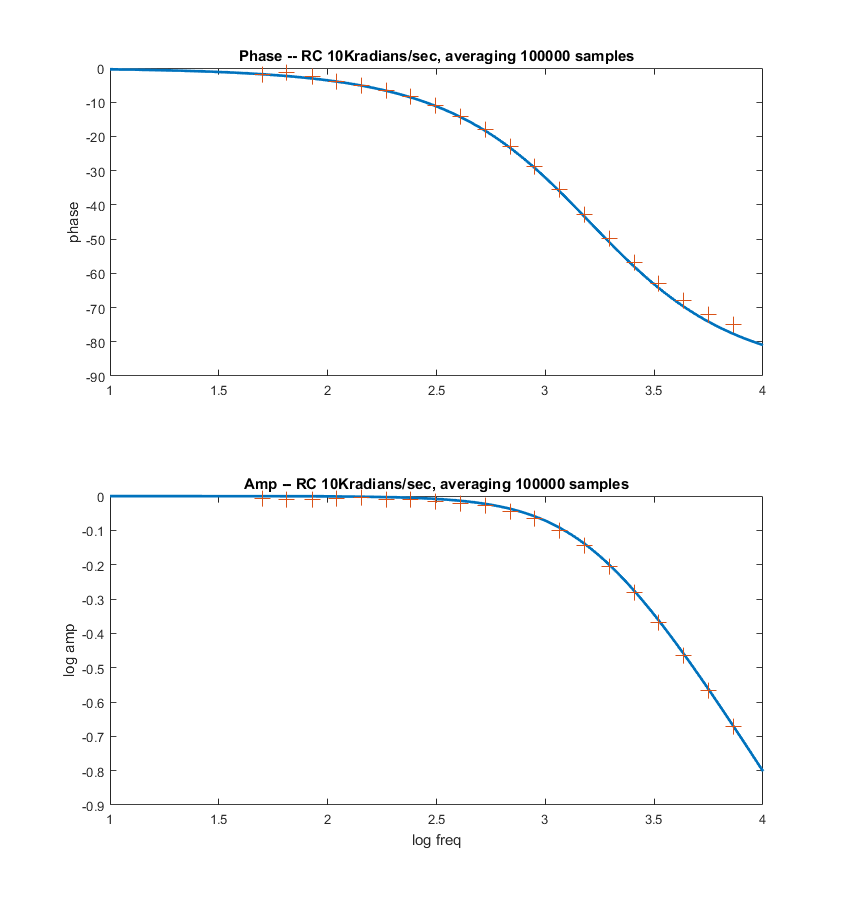
-- A modification of the low pass algorithm allows for much better averaging by adding together up to 200,000 of the quadrature signals, representing an average of the measurements for up to one second. More points means accuracy at lower frequency. Averaging 50,000 points works down to about 100 Hz, 200,000 works down to lower than 5 Hz. There is a systematic phase error which can be calibrated out. The SPI transaction is ends in the ISR following the ISR where it started. That implies a 5 microsecond delay in the DAC update, and thus a frequency-dependent phase-shift. Also, as the frequency increases, the sine approximation gets worse using DDS. The phase correction is linear in frequency and corresponds to 5 degrees/KHz. Code. The first two plots below compare the theoratical curves (in Matlab) with the data generated by the program, shown as '+' symbols. Modifying the frequency-dependent phase correction from f_main*0.005 to f_main*0.0048 makes the phase fit better in the third image. Addition of a scan command (code) produces a table of frequencies, phases, and amplitudes to feed to matlab.
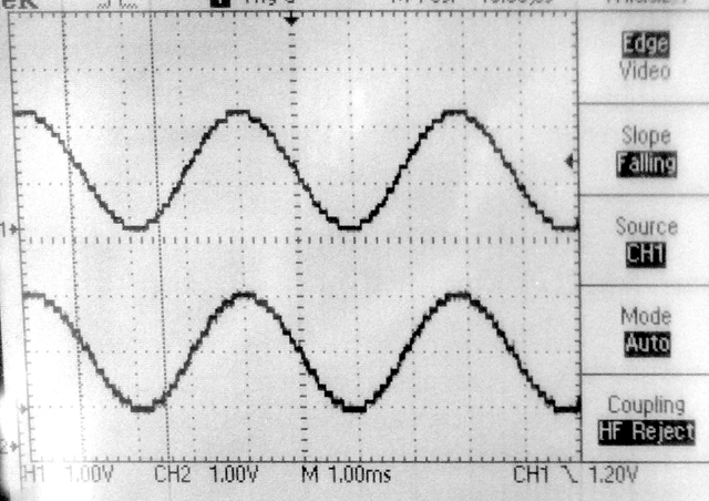
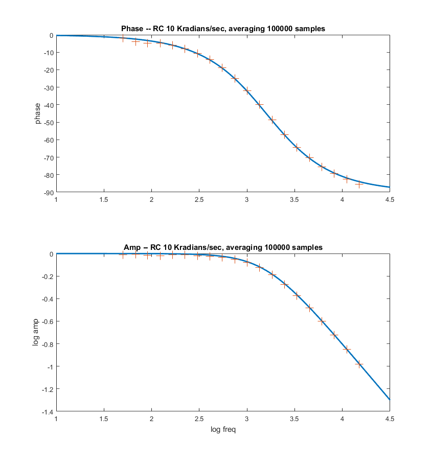
-- Adding a lowpass filter with a time constant of 3 microseconds to the sinewave output (200 KHz sample rate implies 5 microsecond sample time), and recording both the input and output of the circuit-under-test (CUT) drops the error to below 0.25 degrees/KHz. The phase of the CUT is then output phase minus input phase, and the gain is the ratio of output/input amplitudes. This extends the range of correct phase above 10 KHz, as shown in the 4th plot below. Code

--A variant of this process could be used to make a guitar tuner. The analog input signal is from a microphone. The DDS forms sine waves just below, equal to, and just above the desired frequency. Comparing the cross-correlation over a second or so gives a good frequency estimate. matlab example.
The speech waveform has lots of redundancy, so compression is useful. The filter bank formulation described below was used to analyse speech into a number of log-distributed frequency bands. Historically, this scheme was used as early as 1928 and was called a Speech Vocoder. The energy in each of N filters outputs was sampled at a rate around 128 times slower than the original waveform, then reconstucted using just N pure sine waves with amplitudes adjusted to the N filter amplitudes. The result is a slightly sing-song version of the original voice signal. Sample rate for the audio is 8 KHz. Analysis was done in Matlab, with reconstruction also in Matlab, but also with filter output in a header file to a C program running on the PIC32. A voice sample was analysed and reconstructed using 15 filter channels, or 30 channels, or 8 channels. A version pitch-shifted up 1.75 times, and with 30 channels. The filter power was down-sampled to every 16 milliseconds (approximately one fundamental period). Overall compression is 8:1 from the 8-bit, 8KHz input samples to the 15 sampled filter outputs. The Matlab analyser and reconstruction is here. The C header file writtten by the Matlab program contains the filter coefficients, and some constants that the PIC32 reconstruction program needs. The C program defines N direct digital synthesis units and scales their amplitude according to filter coefficients stored in the header file, then blasts them out to a 12-bit SPI attached DAC. The program runs under ProtoThreads. The spectrum of the reconstructed speech looks nothing like the original but is understandable. A better set of filters appears to be distrubuted from 340 Hz to 3400 Hz. Perhaps 15 to 20 filters in that range works well.
Other approaches to speech compression include:
-- Adaptive Differential Pulse Code Modulation: ADPCM uses the continuity of the waveform to reduce the number of bits by sending an estimate of the first derivitive of the speech waveform.
-- Linear Predictive Coding: LPC uses a parametric model of the speech generation process. The model parameters representing the shape of the throat and mouth are sent at lower rate than the waveform samples. (History of LPC, Linear Prediction and Levinson-Durbin Algorithm , Wideband Speech Coding with Linear Predictive Coding, LPC-10 low bandwidth coding )
-- Speech encoding standards: Speech Coding Methods, Standards, and Applications, VoIP: An In-Depth Analysis
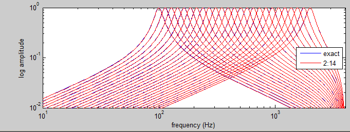
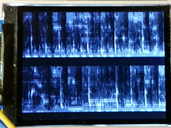
A set of 25, 2-pole, Butterworth, digital filters designed in matlab were converted into GCC using fixed point 2:14 format (14 bit fraction).
The filter responses are shown below. A GCC header file transfers the coefficients from matlab to the GCC program. The GCC program
runs a thread to update the display every 12 milliseconds. One vertical line of intensities is drawn at every update.
The filter responses are computed at every sample time, then each filter output is averaged over about 8 mSec with an absolute value and a low pass filter.
The sample rate is 8 KHz in this code, but could be faster.
The images below show spectrographs of "Smoke on the water" on the left, and a voice sample on the right.
Frequency (actually log(freq)) is on the vertical axis, time on the horizontal axis and loud frequencies are brighter. Time flows across
the top, then the bottom, then back to the top.
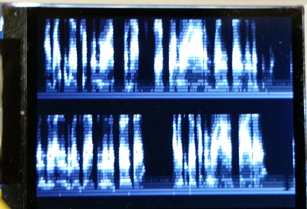
A modification of the timer ISR allows for nonlinear low pass filtering of the bandpass outputs. If the band pass output is louder than the
current low pass output for that filter, then the input is just copied to the output. This allows for fast transients to be recorded.
Code. ZIP of project. Pressing zero on the keypad selects linear mode, pressing one selects fast transient, nonlinear mode.
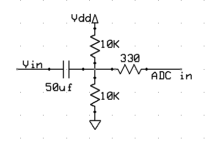
The ADC input is protected by a Vdd/2 voltage divider and capacitor.

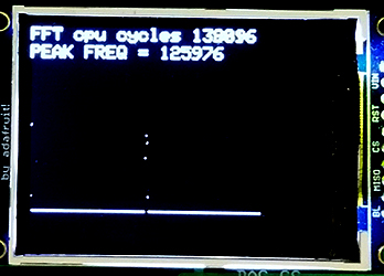
The ADC input was DMAed into RAM then a spectrum was extracted by adding a fixed point FFT routine. The routine works in 2:14 fixed format. A 512 point complex FFT, including the time to Hanning window the signal and compute the log(magnitude) of the complex output, the process takes about 138,000 cpu cycles (at optimization == 1). The magnitude of the FFT is approximated as
|amplitude|=max(|Re|,|Im|)+0.4*min(|Re|,|Im|). This approximation is accurate within about 4%.
Taking the log of the magnitude using a fast approximation
(Generation of Products and Quotients Using Approximate Binary Logarithms for Digital Filtering Applications, IEEE Transactions on Computers 1970 vol.19 Issue No.02) gives more resolution at lower amplitudes.
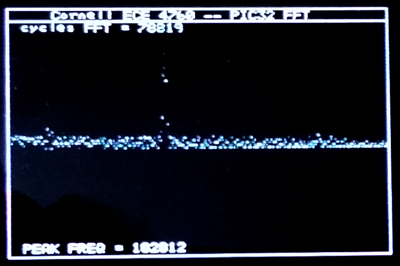
The log was only computed to a 4-bit integer, concantenated with a 4-bit fraction for display at limited TFT resolution. In the first image below, the sampling rate is 500 KHz, and the signal applied was 123 KHz sine wave. You can see the spike of the sine wave as well as the DC offset at zero frequency. (Code) You can get rid of the residual log-noise by truncating at log=0x20 (2 bits in power). The second image shows a calculation of peak frequency. (Code)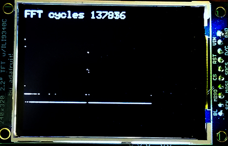
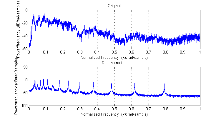
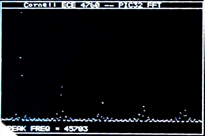
The TV framework described below was used as a spectrum analyser by adding a fixed point FFT routine. The routine works in 16:16 fixed format (but note that the multiply was simplifed based on limited data range). A 512 point complex FFT takes 410,000 cpu cycles (with no optimization) or about 6.8 milliseconds. If we include the time to Hanning window the signal and compute the magnitude of the complex output, the process takes 454,800 cpu cycles (with no optimization), or about 7.6 milliseconds. Running the compiler at optimization level 1 (highest free compiler level) reduces the number of cpu cycles to 146,000, or about 2.4 milliseconds for Hanning-FFT-magnutude calculation. The two images show a sine signal and a square wave captured at 900,000 samples/sec. There is some aliasing of the square wave so the peaks are not clean, but you can see the 1/f spectrum. The magnitude of the FFT is approximated as
|amplitude|=max(|Re|,|Im|)+0.4*min(|Re|,|Im|). This approximation is accurate within about 4%.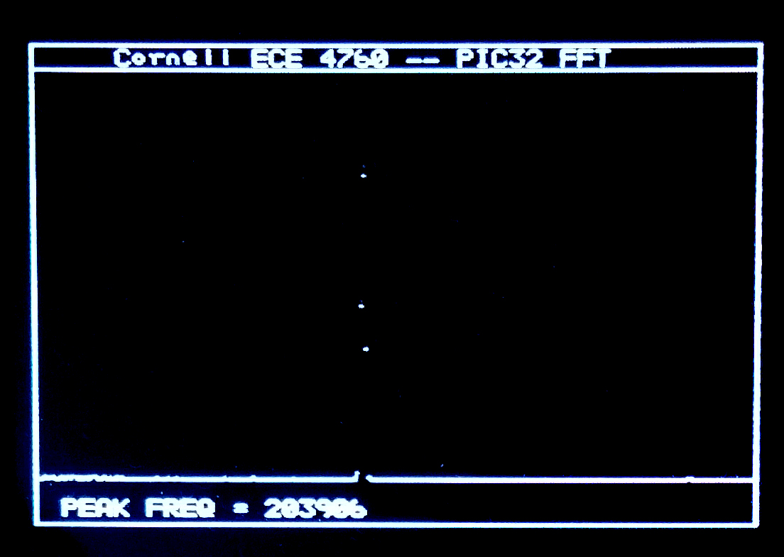
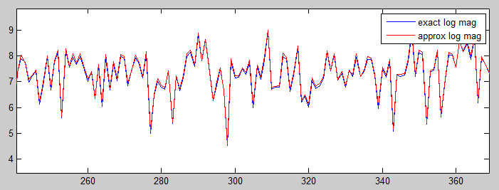
Taking the log of the magnitude using a fast approximation (Generation of Products and Quotients Using Approximate Binary Logarithms for Digital Filtering Applications, IEEE Transactions on Computers 1970 vol.19 Issue No.02) gives more resolution at lower amplitudes( code). Evaluation of the algorithm as a matlab program is here. The following images give the matlab comparison of exact and approximate log for noise, and a sinewave FFT on the PIC32.
I decided to start by implementing Butterworth IIR filters using the fixed point formats below. The first step is to find out how much the limited precision arithmetic will affect the filters. I am not using the PIC32 DSP ligrary because I could not figure out the format for the constants. Filters are implemented as unfactored first or second order Direct forms or as second order sections (SOS) which take a scale factor input as well as two a-vector values. For Butterworth, the b-vector is fixed (refer to Matlab or Octave
butter function). This matlab program allows you to check SOS filter response accuracy for a given bandwidth. This program uses an unfactored IIR filter design for comparision. For low-order filters (one or two samples), unfactored IIR filters will be faster, while being accurate enough. >>>NOTE that all filters in this section use 2.14 format, but the name of the format in the code is fix16.<<<
-- A one-sample (RC type) lowpass filter executes in 89 cycles on the PIC32 as shown in this C program. The filter uses an array for the filter coefficients and another for the filter history. Inserting this filter into the ADC-to-DAC code in a section below results in a program in which the ISR samples the ADC, filters, scales and outputs to the DAC in 2.7 microseconds, including ISR overhead (60 MHz core clock). In this code, the sample rate Fs=100 kHz, the filter cutoff is 0.01/(Fs/2)=500 Hz. Actual cutoff measured in 490 Hz. This filter has less than 1% error above a cutoff=0.002.
// coeff = {b2, -a2} noting that b1=b2 and a1=1 (for first order Butterworth)
// history = { last_input, last_output}
fix16 coeff[2], history[2], output, input ;
fix16 IIR_butter_1_16(fix16 input, fix16 *coeff, fix16 *history )
{
    fix16 output;
    output = multfix16(input+history[0], coeff[0]) + multfix16(history[1], coeff[1]) ;
    history[0] = input ;
    history[1] = output ;
    return output ;
}
-- A second order Butterworth lowpass has less than 1% response error down to cutoff=0.04. At cutoff=0.1 (and Fs=100 kHz) the measured cutoff frequency is very close to 5 kHz, as predicted. The ISR takes 3.5 microSec to execute (60 MHz core clock). -- A second order Butterworth bandpass can be set down to a bandwidth of about 0.003 with less than 1% error. At cutoff=[0.1, 0.11] (and Fs=100 kHz) the measured peask response is 5.25 kHz and the cutoffs are at 4.98 and 5.5 kHz, as predicted. Tthe DC component of the input is removed by the highpass characteristic of the filter, so a DC correction has to be made because the DAC can only produce a positive voltage. In the ISR, 128 is added to the 8 bit DAC value
DAC_value = (output>>6) + 128 ;.-- A generalized SOS Butterworth lowpass executes in 7.5 microSec (ISR, 60 MHz core clock, 4-pole). The 4-pole version with a cutoff=0.1 has the predicted resopnses near the cutoff frequency and where the response drops to 0.1 of peak. Six-pole takes 10 microSec, 8-pole takes 12.5 microSec. The sample frequency is set to 20 kHz. This matlab program computes the filter parameters for SOS and prints C code to the matlab console window to paste into the program for both lowpass and bandpass filters.
-- A generalized SOS Butterworth bandpass filter which uses the matlab progam mentioned just above to construct parameters. The example is set to a bandwidth of 0.002, about as narrow as you can get with 2.14 format fixed coefficients.
-- The SOS filters above are easy to read, but slow to execute because of the 2D arrays. Unrolling the loops, and making all the indices constant, speeds up the filters by almost a factor of two. This program uses the UART interface to profile number of cycles to execute. Putting the revised SOS filters back into the realtime program with ADC and DAC gives an ISR time of 7.7 microSec for the 4-section, eight-pole, bandpass filter. Almost all of the time in the ISR is the filter. A reasonable rule would be 2 microSec/pole of filtering. At 8 kHz sample rate, could do about 60 poles of filtering, or about fifteen 4-pole filters.
-- Fixed point arithmetic is the first step to building DSP functions. I decided to implement 2.30 and 2.14 formats. This means two bits to the left of the binary-point, one of which is the sign bit. The dynamic range of the systems is either -2 to 2-2-14 or -2 to 2-2-30. The resolution is either 2-14=6*10-5 or 2-30=9*10-10. The resolution is necessary to make stable, accurate, filters. The dynamic range is sufficient for Butterworth, IIR filters, made with second order sections (SOS). SOS help to minimize filter roundoff errors. This program defined the data types and macros for converting float-to-fix, fix-to-float and fixed point multiply. Add and subtract just work. The program uses timer2 to count cycles to profile the time for the add and multiply operations, then uses the UART (see section below) to print the results. The 2.30 format takes 40 cycles to to a multiply-and-accumulate (MAC) operation. The 2.14 format takes 17 cycles for a MAC operation (level 0 opt). The 2.14 result (
1.5*0.05-0.25) is in error by 4*10-5, the 2.30 result is correct to 8 places. The macros for the 2.30 follow:
typedef signed int fix32 ;
#define multfix32(a,b) ((fix32)(((( signed long long)(a))*(( signed long long)(b)))>>30)) //multiply two fixed 2:30
#define float2fix32(a) ((fix32)((a)*1073741824.0)) // 2^30
#define fix2float32(a) ((float)(a)/1073741824.0)
Another fixed point system useful over a larger integer range is 16.16 format with a range of +/-32767 and a resolution of 1.5x10⁻⁵. The macros for this system are
typedef signed int fix16 ;
#define multfix16(a,b) ((fix16)(((( signed long long)(a))*(( signed long long)(b)))>>16)) //multiply two fixed 16:16
#define float2fix16(a) ((fix16)((a)*65536.0)) // 2^16
#define fix2float16(a) ((float)(a)/65536.0)
#define divfix16(a,b) ((fix16)((((signed long long)(a)<<16)/(b))))
#define sqrtfix16(a) (float2fix16(sqrt(fix2float16(a))))
The performance for operations vary. At level 1 opt, fixed multiply is about 2.4 times faster than floating point (23 cycles), and fixed add is about 8 times faster (8 cycles). However fixed divide is the same speed as float, and fixed square root is 0.6 the speed of the float operation. Test code.
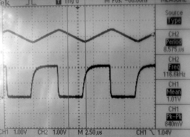
-- The Vref generator can be connected to an external pin (pin 25 on PIC32MX250F128B) and can be set to 16 values between zero and two volts. The first example generates a 16-sample square wave to investigate the settling time of the DAC. According to the Reference Manual, the output impedance at output level 0 (about zero volts) is about 500 ohms, while the output impedance at output level 15 (about 2 volts) is around 10k ohms. The first screen dump shows the Vref voltage output on the bottom trace and the same signal passed through an LM358 opamp, set up as a unity gain impedance buffer, on the top trace. Rise time (level 15) is about 0.5 microSec (to 63%) and fall time (level 0) is about 0.05 microSec. The rise/fall times are dominated by the RC circuit formed by the output impedance of Vref and the capacitance of the white board (10-20 pf) and the scope (20 pf). The LM358 is slew-rate limited and thus produces a triangle wave.
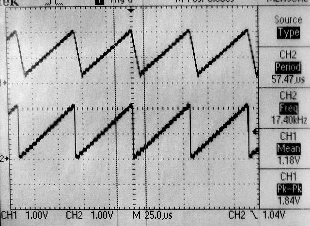
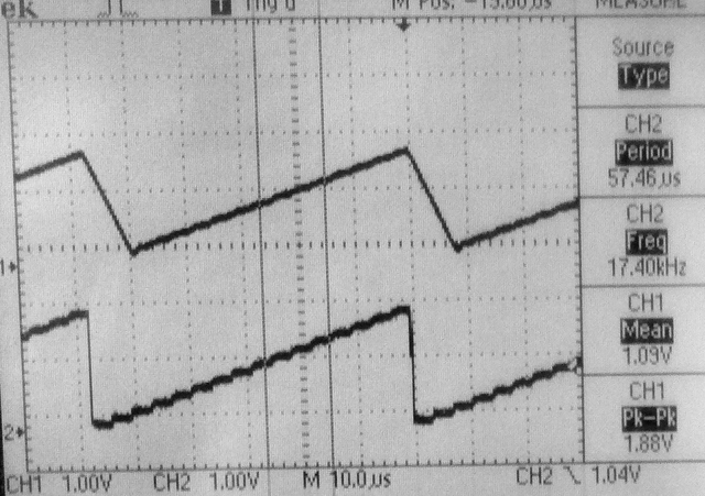
-- The next example generates a sawtooth with a period of 128 phase increments (17.4 kHz). The bottom trace is taken directly from the Vref pin, while the top trace is from the output of the unity gain LM258 follower. Notice the slew-rate limiting on the falling edge of the sawtooth.To unload the Vref pin, the output was connected to the opamp follower through a 100k resistor. A lowpass filter using the 100k resistor and a 10 pf capacitor with a time constant of around 1 microSec smooths and denoises the opamp trace (third image).
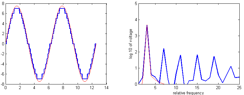
-- Any real application is going to use ISR-driven timing to output samples to the DAC. The next example uses Direct Digital Synthesis (DDS) running in an ISR at 100 kHz to generate sine waves. Tiiming the ISR using a toggled bit in MAIN, suggests that the 47 assembler instruction ISR executes (with overhead) in 1.5 microSeconds. The first image shows the DDS sine wave (but at very high frequency) on the top trace and the bit being toggled in MAIN on the bottem trace. You can clearly see the 1.5 microsecond pause in MAIN every time a new sine wave value is produced. The second image is a sine generated at Middle C (261.6 Hz). The top trace in the lowpassed opamp output. The bottom is the raw Vref pin.The code is structured as a timer ISR running the DDS. The output frequency is settable within a millHertz, but accuracy is determined by the cpu clock. Sixteen voltage levels introduces some harmonic distortion. The first error harmonic is about a factor of 30 in amplitude below the fundamental and at 3 times the frequency. This is in line with Bennett for 4-bit signals. The matlab image shows the full and 16-level sampled sine waves on the left and their spectra on the right (code). Listening to the signal gives a sense of very high frequency spikes. Lowpass filtering with a time constant equal to about 1/(sample-rate) gets rid of most of the sampling noise..