Cornell University ECE4760
Spiking Neural Models
PIC32MX250F128B
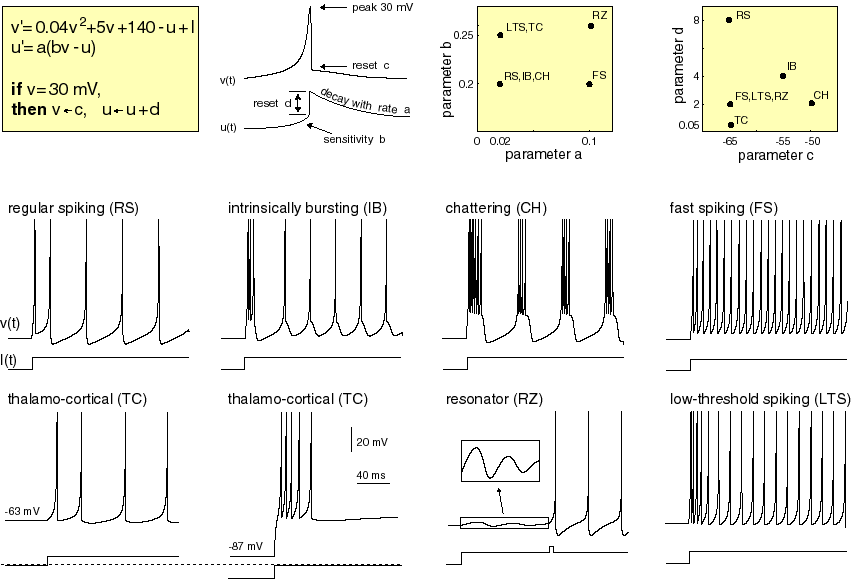
Izhikevich Neural Model:
The Neuron
Eugene Izhikevich developed a simple, semiempirical,
model of cortical neurons. The properties of each neuron are controlled by 4 parameters, plus a constant current input. His web site includes matlab programs and detailed descriptions of the cell model. There are two state variables: v is the membrane potential and u is the membrane recovery variable. The differential equations, parameter settings and examples of model output are shown below in a figure from Izhikevich's web site. An electronic version of the figure and reproduction permissions are freely available at www.izhikevich.com. The model belongs to the class of reduced Hodgin_Huxley models, much like the FitzHugh-Nagamo model, but simpler to compute. The model has reasonable dynamic properties near threshold (unlike integrate-and-fire models). Stability is maintained through resetting the state variables when the positive feedback pushes the voltage to the "action potential peak".
Implementation on PIC32
The equations above were scaled to use 2:14 fixed point arithmetic and the constants a and b were converted to simple shifts to minimize multiplications.Note that v and u are scaled down by a factor of 100 so that the dynamic range is -1 to +1, as required by the arithmetic system. Compared to the equations above, the scaled equations have all constant terms divided by 100. The a and b constants are not scaled (because they are multiplied by the scaled variables), but c and d are divided by 100. The constant (.04) on the v2 term above is scaled up by 100 because squaring (the scaled) v drops the value by 10,000. The final scaled equations are:
v1(n+1) = v1(n) + dt*(4*(v1(n)^2) + 5*v1(n) +1.40 - u1(n) + I)
u1(n+1) = u1 + dt*a*(b*v1(n) - u1(n))
if (v1>=0.30) {v1=c; u1=u1+d}
Now we set dt to a factor of two (say 1/16). We actually code as below (for neuron i) where c14 = float2fix14(1.4/4) and
the multiply by dt is replaced by a right-shift.
However, in thee voltage update equation, the 4-bit right-shift is factored into a divide-by-4 (to scale the factors of 4 and 5 above to 1 and 1.25), followed by another divide-by-4
(2-bit shift).
v[i] = v[i] + ((multfix14(v[i],v[i]) + v[i] + (v[i]>>2) + c14 - (u[i]>>2) + ((Is[i]+I_syn[i])>>2))>> 2);
u_reset[i] = u[i] + d[i];
u[i ] = u[i] + ((((v[i]>>b[i])-u[i])>>a[i])>>4);
If a spike occurs then u and v are reset.
if(v[i] > peak){ v[i] = c[i] ; u[i] = u_reset[i] ; spike[i] = 1; }
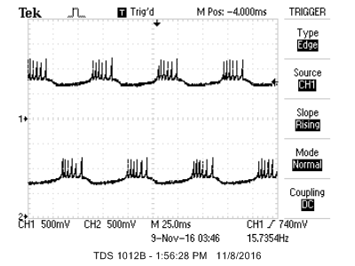
-- The first example has a network of 20 tonic bursting neurons (type 3 -- see table below) with arbitrary connections, so there are 400 synapses. For testing, most of the synapse weights are set to a low, random value. Synaptic current has a instant rise and exponential fall. The serial user interface allows you to display any two of v[i] through a DAC (also see DSP page) to a scope. In the example neurons 1 and 2 are reciprocally connected with negative weights, so that they alternate bursts, as shown below. You can optionally turn on spike-time-dependent-learning (STDL) by uncommenting a macro. STDL changes the weight of a synaptic connection depending on whether the postsynaptic spike follows (causal) or leads (non causal) the presynaptic input spike. Causal connnections are made stronger, noncausal weaker. Speed of execution is determined by the number of neurons, number of synapses, and optionally STDL. The STDL computation approximately halves the number of neurons computed in real-time.
-- Updated for the SECABB big board and Protothreads 1.3.0, with 2 SPI DAC readout channels,
TFT display of all neurons and serial terminal interface to set parameters
through a simple command language.
(code, zip)
The image shown is for 10 type-3 burster neurons with random, weakly-weighted,
connections between them.
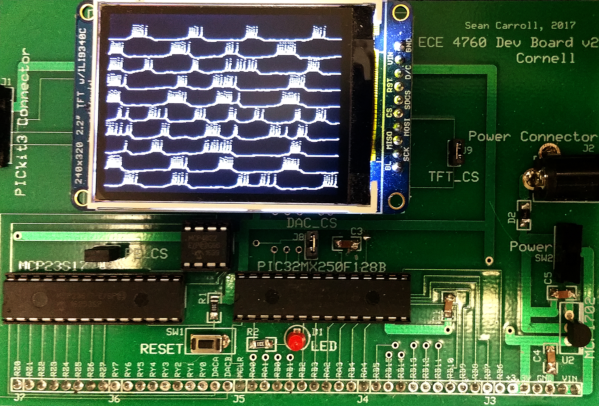
Table of neuron behavior types, from Izhikevich web page, but note scaling of a,b,c,d and Is for the C code above.
 %cell parameters from Izhikevich web page
 * in the CODE:
 * --a from this table converted to a approx right shift number so 0.02 becomes 6
 * --b from this table converted to a approx right shift number so 0.25 becomes 2
 * --c from this table is multiplyed by 0.01
 * --d from this table is multiplyed by 0.01
 * --Is from this table is multiplyed by 0.01
 * For example, the C-code scaling for type 3: a=6, b=3, c=-0.50, d=0.02, Is=0.15
 *
 * % a        b        c      d        Is   index
    0.02      0.2     -65      6       14   0     % tonic spiking
    0.02      0.25    -65      6       0.5  1     % phasic spiking -- Izhikevich type2
    0.02      0.2     -50      2       15   2     % tonic bursting -- Izhikevich type3
    0.02      0.25    -55     0.05     0.6  3     % phasic bursting
    0.02      0.2     -55     4        10   4     % mixed mode
    0.01      0.2     -65     8        30   5     % spike frequency adaptation
    0.2       0.26    -65     0        0    6     % Class 2
    0.02      0.2     -65     6        7    7     % spike latency
    0.05      0.26    -60     0        0    8     % subthreshold oscillations
    0.1       0.26    -60     -1       0    9     % resonator
    0.03      0.25    -60     4        0    10    % rebound spike
    0.03      0.25    -52     0        0    11    % rebound burst
    0.03      0.25    -60     4        0    12    % threshold variability
    1         1.5     -60     0      -65    13    % bistability
    1       0.2       -60     -21      0    14    % DAP
    0.02      1       -55     4        0    15    % accomodation
Copyright Cornell University November 13, 2018