Cornell University ECE4760
Sliding Windowed Infinite Fourier Transform (SWIFT)
Pi Pico RP2350
Page Organization: Contents
The SWIFT algorithm to do a Fourier Transform was so new to me that I needed to build up intuition for how it worked and what it could do. The process invovled writing a description of the math followed by a series of programs.
SWIFT algorithm.
The SWIFT algorithm is a Fourier transform technique which updates the transform at every input sample time, rather than computing a transform on a block of samples, like the FFT. SWIFT also uses an exponentially weighted window, and hence has an infinitely wide window, unlike the finite window of the FFT. These features have several very handy consequences:
Each transform frequency bin, at frequency ω, is computed as a damped, complex resonator, with a real input. The estimate of the frequency bin amplitude at time n is Xn(ω) which is, of course, a complex value. Xn(ω) is computed iteratively from the n-1 time step estimate by slightly decaying the complex amplitude toward zero, advancing the phase by one time step, then adding the real input sample.
Xn(ω) = e(-1/τ) × e(jω) × Xn-1(ω) + xn
The units of ω are radians per sample time,
ω=2*π*F/Fs.
Fs is the sample rate and F is the frequency of the transform bin in Hz.
The decay time constant, τ, has units of number of samples. The time constant determines the bandwidth of the bin. Bigger time constant means narrower bandwidth. Typical values might range from 20 to 100, but could be different for each frequency bin. For speech, τ(ω)=3*Fs/F seems to work well.
Since both τ and ω are constants, the exponentials can be computed once and stored in a table. The real-time computation reduces to one complex multiply and one real add per sample. The transform noise level can be significantly lowered with a better window consisting of two exponentials. This doubles the arithmetic. In the paper linked above this is refered to as the α-SWIFT version, which is what I actually implemented. The α-SWIFT algorithm is:
Xn(ω)α = Xn(ω)slow - Xn(ω)fast
The only difference between the fast and slow spectral estimates is the value of τ Where τslow > τfast > 0. The fast time constant is set to a few samples. The slow time constant is set as above. The overall effect of the two time constants is to reduce spectral leakage by removing the discontinuity in the window when new samples are added.
Example of speech analysis and re-synthesis.
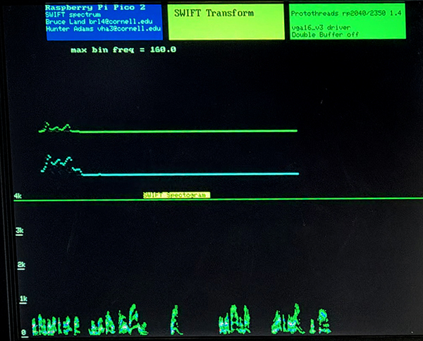
The speech example runs at a sample rate of 10,000 samples/sec. Most of the energy in speech is below 4 KHz, and above ~100 Hz. For testing I transformed the signal into 200 bins from 0 to 4 KHz, with 20 Hz bin spacing. The resulting spectrum, log spectrum and spectrogram was displayed on the VGA. The spectrogram time slice is around 20 milliseconds.
The signal is high-passed at around one Hz to remove residual DC offset. Input comes from a line-level output from a computer. Since the spectral estimate of each frequency is computed as a time-varying phasor, a reconstruction of the original signal was made by summing the time-varying real parts of all the frequency bins and feeding the scaled result to a DAC. This is just a audio loop-back to show everything is working. The sampling ISR, which computes the α-SWIFT and the inverse uses about 0.6 of one cpu at 150 MHz.
Animation of SWIFT algorithm
SWIFT computes the Fourier transform for each frequency separately, just as the DFT does. Unlike the DFT, the correlation between the complex frequency and the input is computed sample-by-sample, with a exponentially decreasing weight for older samples. One way to think of this is to consider the current transform estimate for a given frequency to be a slowly-decaying phasor rotating at that frequency. The next input real-valued sample is just added to the phasor at whatever the phasor's current phase happens to be. The video below shows an input sine wave with frequency of 0.02 radians/time step applied to five complex phasor resonators. The phasor is shown as a rotating white line. The real input is shown as a horizontal yellow line oscillating left-right. The output waveform is the real part of the phasor polotted vs time. You can see that the output of the center phasor becomes much greater than the other because the input freqeucy is always leading the phasor, and therefore driving it to higher amplitude.
This scheme requires about eight real adds and eight real multiplies per computed transform frequency, per time sample. It is thus less efficient in terms of cycles compared to FFT, but has several advantages. The main advantage is that it is completely real-time, so there are no FFT block artifacts resulting from artificial block boundaries. Another advantage is that the bandwidth of each trasformed frequency can be set to a different bandwidth, unlike the FFT which is constrained by the number of points in a block and the block duration. The time constant of the exponential weighting function sets the bandwidth. Longer time constant means narrower bandwidth, the usual time/frequency tradoff. Also, since the exponential window is infinite, the values of the transform frequencies are not quantized. The FFT frequency increment is fixed at the reciprocal of the block duration.
The program has a double-buffered animation thread and a serial thread. The serial thread recognizes several commands to control the graphics display. There are commands to
Investigating the decay-time vs bandwidth tradeoff.
The bandwidth of each transformed frequency can be set to a different bandwidth, by setting the time constant of the exponential weighting function. Generally, a longer time constant means narrower bandwidth. But to get more specific, let's define bandwidth as the Full-Width-Half_Maximum (FWHM) of a given frequency peak, where FWHM means the width of the peak in Hz, at half its maximum amplitude. For the α-SWIFT version, the relevant parameters which determine the bandwidth are the frequency of the peak, the time constant of the exponential decay (slow time constant), and the time constant of the exponential rise function (fast time constant).
The observations are:
Bandwidth program
The bandwidth testing program allows you to enter the relevant parameters for an array of frequency bins, then measures the FWHM for two test frequencies set by a pair of direct digital synthesis (DDS) input sinewaves. Using serial input you can set:
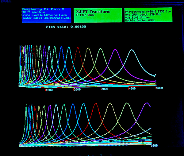
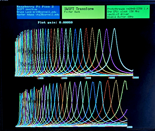
The top half of the screen displays the amplitude spectrum. The bottom half displays the various input parameters and the resulting FWHM for each peak. The first image shows a fixed decay time of 100 samples. Each frequency bin has the same fairly narrow bandwidth, like you would get with a DFT. The second image shows a relative decay time set to 10 times the period of each different frequency. The bandwidth scales with frequency, like you would get with constant Q filters. As the FWHM gets larger, the peak has to drop to satisfy Parseval's theorum.


Designing a Filter Bank
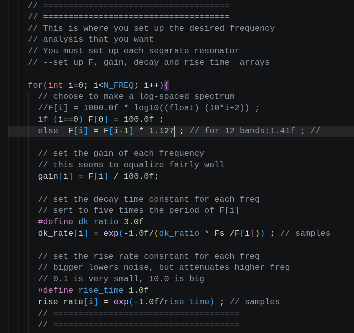
The previous example shows how to design the filter response of a uniformly spaced array of resonators (frequency bins). Most real examples need finer control of each bin. For example speech analysis typically uses frequency bins which are distributed along the frequency axis at log-linear intervals. Each bin can have a different bandwidth and gain, and may need control of the rise time constant. There are so many combinations of layouts and parameters that the filter bank must be defined by changing a small section of the program.
My speech code specifies:
The top trace runs from 0 to Nyquist frequency of 5 KHz.
The bottom trace just expands out the part from 0 to 1000 Hz.
Using SWIFT to build a speech phase-vocoder
A phase vocoder is used to pitch-shift speech or to change speech rate. The SWIFT algorithm can be used to extract the amplitude/phase spectrum of a speech signal. The phase spectrum is used to set the frequency of a multichannel DDS synthesizer, and the amplitude spectrum sets the gain of each DDS channel. The phase difference between two successive samples for a given frequency analysis bin yields the instantaneous frequency content of the bin. This phase change is then Euler integrated to give a phase value that can act as the index into a DDS sinewave lookup table. The sum of the sinewaves from each bin, weighted by the amplitude spectrum, becomes the output signal. If you scale the phase change by a constant near one, then you pitch-shift the output. Practically speaking, the useful pitch shift range is about 0.5<shift-value<2.0. Lower shifts become subsonic and hard to hear. HIgher shifts will start to alias. Both extremes seem to limit intelligibilty.
This example does a settable pitch shift. The 48 bin SWIFT analysis is running in a ISR at 20 KSamples/sec. The same ISR is also computing the instantaneous frequency of each bin output. This may not be the same as the bin center frequency because of the relatively wide bandwidth of each bin. The phase difference between consecutive samples of each bin output is an estimate of the first derivitive of the phase, which is the current frequency. This phase derivitive may be scaled to shift the frequency, and is then fed into an numerical integrator to get the phase for a direct-digital-synthesis (DDS) sine wave generator. The sum of the sine outputs from the 48 DDS units is the vocoder output.
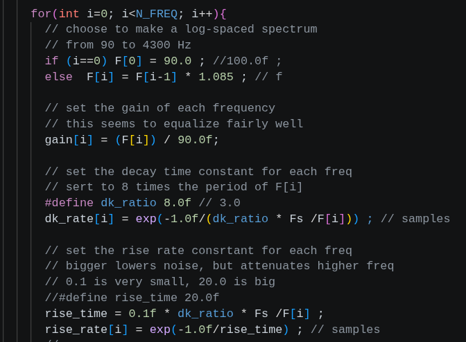
The 48 bins are equally spaced by a frequency ratio of 1.085 from 90 Hz to about 4300 Hz. This range captures most of the energy in human speech. The bandwidth of each bin is set to overlap the next bin at around 40% of peak. The gain of each bin drops somewhat at lower frequency. Every parameter can be modified if you don't like the sound. The filter bank program above was used to design the vocoder bins
Sound Samples:
Original voice sample from an old lecture.
Shifted down to 0.8 of original pitch.
Shifted up to 1.4 of original pitch
The program is organized as two threads running on one core, and one ISR running of the other core. One thread precomputes and stores all of the complex constants necessary for efficient arithmetic in the ISR. The other thread is a simple serial interface to a terminal emulator used to set the pitch shift.
For each sample time, the ISR:
The rp2350 has single precision float hardware. Double precision is slow because the operations are emulated in hardware/software.
For speed sensitive routines, it is important to remind the C compiler that you want single precision floating point:
Copyright Cornell University July 22, 2026