We will consider three types of filters in two catagories:
- Those which simulate electronic filters:
- Butterworth filters which have optimal flat frequency response.
- Chebychev type 1 filters which have good frequency cutoff response.
- In general, these filters are refered to as infinite-impulse response filters because a pulse input can produce a (small) lingering output for a long time.
- Those which are optimized for computers
- Convolution filters designed by the Parks-McClellan scheme.
- In general, these filters are refered to as finite-impulse response filters because there is a definite time beyond which the output is exactly zero after a pulse is applied.
We will look at the effect of these three filters on three different time series:
- A single square pulse. It is easy to see how a filter distorts risetime using a pulse. It is also easy to see how a filter reduces the noise on the pulse.
- A chirped sine wave, which is a sine wave of increasing frequency. It is easy to see how a filter cuts off certain frequencies using a chirped sine.
- A simulated miniature endplate potential. This is a pulse-like time series of relevance to neurobiology.
The GUIfilter.m program allows you to see the effects of all combinations of the above inputs and filters. Two screen shots are shown below. The first screen shot shows the input/output of a filter, The second show the filter's frequency response. Click either one for more detail. For those who don't like graphical interfaces (or who want to use the code for something else) there is a version with absolutely no user interface, but which calculates the same functions.
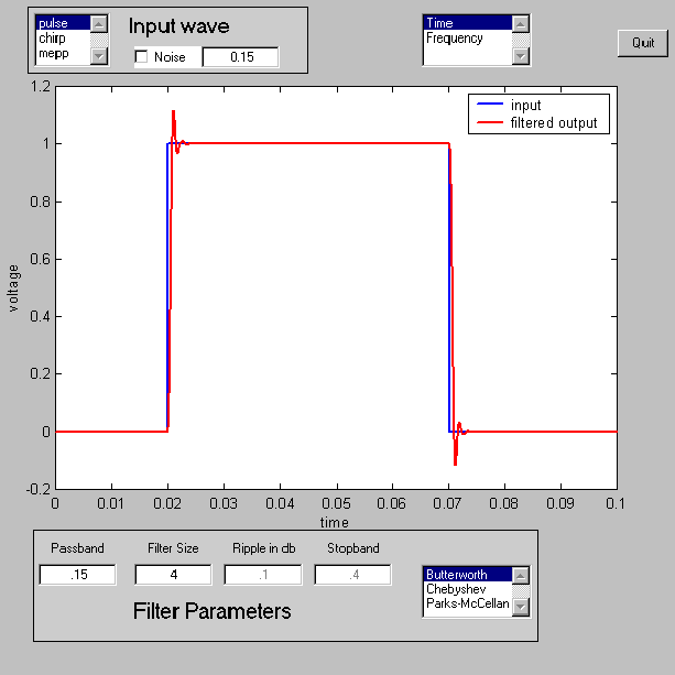

The filters are controlled by the four filter parameters:
- The passband control sets the frequency at which the filter starts to attenuate the signal. Passband units are 0-1 where 1 corresponds to the Nyquist frequency.
- The stopband control sets the frequency at which the Parks-McCellan scheme cuts off all the signal. The units are the same as the passband control.
- The filter size control is used to determine how many input samples are used to compute one output sample. Typical sizes for Butterworth and Chebychev filters are 2 to 8. Typical sizes for the Parks-McCellan scheme are 11 to 121.
- The ripple control sets the amplitude error in the passband for Chebychev only.
- After setting the filter parameters, be sure to select the frequency display to show the actual filter response.
Observations:
- For all designs:
- Decreasing the passband distorts the output by removing fast transitions. This effect is most obvious for the pulse input.
- Decreasing the passband reduces the noise level (if noise is turned on).
- The optimal passband is always a tradeoff between noise reduction and signal distortion.
- Increasing the number of samples causes a delay in the output signal. This means that filtering distorts arrival-time information, which could be significant for studies of action potentials where information is carried by the spike arrival time.
- For Butterworth designs:
- Bigger filter size means faster frequency cutoff, but more overshoot on pulses.
- The amplitude of the pulse is very accurate after the initial rise time.
- Using the chirp input will show that this filter has a very flat frequency response at low frequency. This means that it is good for obtaining the relative size of low frequency waves.
- For Cheychev designs:
- Bigger filter size means faster frequency cutoff, but more overshoot on pulses.
- The accuracy of the amplitude of the pulse depends on the value of the ripple. Smaller ripple means better accuracy. But choosing an filter with an odd number of points results in good accuracy independent of the ripple setting.
- The value of the ripple also effects the overshoot at the beginning and end of a pulse. The value of the ripple sets the maximum size of deviations from flat frequency response, thus relative amplitudes of different frequency waves may be distorted.
- It is probably reasonable to not use Chebchev designs when the goal is fidelity of pulses.
- For Parks-McCellan designs:
- The effect on a pulse is almost entirely a delay if there is enough difference between the passband and stopband values (and the filter size is big enough). This is probably the filter of choice for pulses.
- Small filter sizes lead to gross amplitude errors.
- There is ripple in both the passband and the stopband.
- This program does not demonstrate all of the flexibility the Parks-McCellan design scheme can perform.
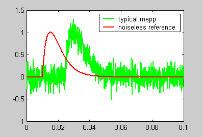
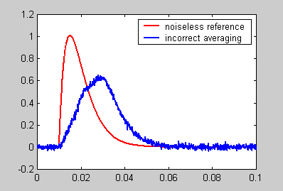
In the analysis program, we want to estimate the amplitude, rise time and fall time of the noise-corrupted mepp. We can't just average the traces together because they are not aligned in time. Each mepp starts at a time between 100 and 300 samples into the recording. A simple, but incorrect, program produces the following result. Notice the modified shape and slow risetime of the averaged trace.
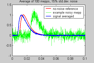
The final version of the program aligns the mepps, then averages them. The alignment process includes:
- Estimate the peak for each mepp
- Fit the points near the peak to a quadratic curve
- Re-estimate the peak from the maximum of the quadratic
- Filter the original mepp and find the point which is in the rising phase, and equal to 1/2 of the peak.
- Shift the original, unfiltered mepp so that the 1/2 point is at a standard position.
The result is shown below. Note that the averaged trace has virtually the same shape as the noise-free reference.