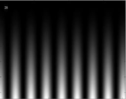
clf
clear all
set(gcf,'doublebuffer','on');

%Build the grid which determines the image resolution
[x,y] = meshgrid(1:256,1:128);

%initialize the movie
n=40;
mov=moviein(n);

%build the frames
speed=.05;freq=.2;
for i=1:n
   %the frame is just a sinewave grating
   %intensity modulated to--to-botton
   img=128 * (sin(x*freq+speed*i)+1) .* y.^2/128^2;
   image(img);
   %add a frame number
   text(10,10,num2str(i),'color','white')
   %Force real pixels
   truesize(gcf)
   %transfer the image to a movie frame
   mov(i)=getframe;
end

%clear the image
image(0*x);axis image;
pause(1);
%playback the movie
%--five times, with reversal
%--at 30 frames/sec
movie(mov,-5,30);
image(0*x);axis image;
One frame from the animation is shown below.
% generate a fractal coastline via FFT
clf;
clear all;
%grid size
n = 256;
[x,y] = meshgrid(1:n,1:n);
%Generate a random frequency domain grid
s = sum(100*clock);
rand('seed',s);
freq = (rand(n,n)-.5) + i* (rand(n,n)-.5);
% Set the DC level to zero
freq(1,1) = 0;
% Slope of cutoff filter in freq domain
%less negative => rougher outline
%-1.5 to -2.5 is reasonable for real coestlines
c = -2.1;
%
% make a matrix with entries proportional to the freq
dist = sqrt( x.^2 + y.^2 ) ;
% Reduce high freq components by a power law f**c
%to make a fractal surface
filtered = freq .* dist .^c ;
surface = ( real(ifft2(filtered)) ) ;
%add a bias to make a lake or a mountain
%just change the sign when adding the bias to the surface
bias = 6e-8*sqrt( (x-n/2).^2 + (y-n/2).^2 );
bias = bias-mean(mean(bias));
surface = surface - bias ;
%Convert to a rgb (truecolor) image
surface = cat(3,...
.8*(surface>0), ...
.6*(surface>0),...
surface<=0);
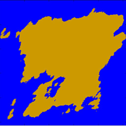
image(surface);
truesize(gcf);
An example is shown below.
figure(1)
clf;
set(gcf,'doublebuffer','on')
clear all;

%grid size
n = 128;

%Generate a random frequency domain grid
s = sum(100*clock);
rand('seed',s);
freq = (rand(n,n)-.5) + i* (rand(n,n)-.5);
%Set the DC level to zero
newfreq(n/2,n/2) = 0;

%low pass parameter--bigger means faster pattern
alpha = .1;
%lowest spatial frequency -- units are cycles/frame width
lowcut = 2;
%highest spatial frequency
hicut = 10;

% make a matrix with entries proportional to the freq
%for use in filtering in freq domain
[x,y] = meshgrid(1:n,1:n);
dist = sqrt( (x-n/2).^2 + (y-n/2).^2 ) ;

for j=1:120
    %get the next random input
    newfreq = (rand(n,n)-.5) + i* (rand(n,n)-.5);
    % Set the DC level to zero
    newfreq(n/2,n/2) = 0;
    %lowpass filter combines old and new state
    freq = freq *(1-alpha) + newfreq*alpha;

    %band-pass filter the spatial frequency
    filtered = freq .* ( (dist>=lowcut) & (dist<=hicut) );

    %make the intensity distribution
    surface = abs( (ifft2(fftshift(filtered))) ) ;
    %and scale it to 0-1 range
    surface = (surface - min(min(surface)))/(max(max(surface)) - min(min(surface)));

    %Convert to a rgb (truecolor) image
    dis = cat(3,surface, surface, surface);
    %display the grayscale image
    imshow(dis);
    truesize(gcf);
    colormap(gray);
    mov(j) = getframe;
    %drawnow
end

figure(2)
movie(mov,1,30);
%make two animal distibutions
dist1x=randn(100,1);
dist1y=randn(100,1);
dist2x=randn(100,1)+2;
dist2y=randn(100,1);
%compute the convex hull of each
c1=convhull(dist1x,dist1y);
c2=convhull(dist2x,dist2y);
%plot the two distributions and
%their respective convex hulls
figure(1)
clf
hold on
plot(dist1x,dist1y,'r.');
plot(dist1x(c1),dist1y(c1),'r');
plot(dist2x,dist2y,'b.');
plot(dist2x(c2),dist2y(c2),'b');
%will need the image size below
xdist=get(gca,'xlim');
ydist=get(gca,'ylim');
%=============
%fill the convex hull polygons
%convert them to binary images
%then compute the intersection area
%and compute the area ratios
figure(2)
clf
hold off
axis image
fill(dist1x(c1),dist1y(c1),'r');
set(gca,'xlim',xdist);
set(gca,'ylim',ydist);
pause(1)
img=getframe;
d1bw=~im2bw(img.cdata,.9);
imshow (d1bw);
pause(1)
fill(dist2x(c2),dist2y(c2),'r');
set(gca,'xlim',xdist);
set(gca,'ylim',ydist);
img=getframe;
d2bw=~im2bw(img.cdata,.9);
imshow (d2bw);
pause(1)
%trim the image edges because of
%bogus pixels at the edges
[a b]=size(d1bw)
d1bw=(d1bw(5:a-10,5:b-10));
d2bw=(d2bw(5:a-10,5:b-10));
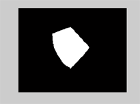
imshow(d2bw & d1bw)
disp('areas')
bwarea(d2bw & d1bw)
bwarea(d2bw & d1bw)/bwarea(d2bw)
bwarea(d2bw & d1bw)/bwarea(d1bw)
An example of two disributions and their computed overlap region is shown
below.