Neuron Models on FPGA
We can use the FPGA to do fast numerical integration to solve differential equation models of neurons. This page describes a couple of neuron models and their solution by DDA techniques. The Digital Differential Analyzer (DDA) is a device to directly compute the solution of differential equations. See the DDA page for more algorithm and numerical details.
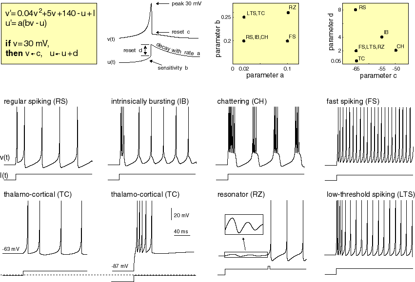
Izhikevich Neural Model:
The Neuron
Eugene Izhikevich developed a simple, semiempirical,
model of cortical neurons. The properties of each neuron are controlled by 4 parameters, plus a constant current input. His web site includes matlab programs and detailed descriptions of the cell model. There are two state variables: v is the membrane potential and u is the membrane recovery variable. The differential equations, parameter settings and examples of model output are shown below in a figure from Izhikevich's web site. An electronic version of the figure and reproduction permissions are freely available at www.izhikevich.com.
Implementation on the CycloneII
The model consists of several verilog modules which include (see also Ruben Guerrero-Rivera, et al below):
- Soma model (cell body and spike generator)
- Time constant of 16 time steps (nominal time step of 1/16 mSec)
- Square-law dynamics (as explained in the History section below)
- Settable a, b, c, d, and I parameters (as explained in the diagrams above)
- Spike propagation delay (axon)
- Delays of 1 to 64 time steps to simulate movement of a spike along an axon connection.
- Chemical Synapse
- Constant current source gated by an presynaptic action potential.
- Exponential fall time constant settable at 4, 8, 16, 32, 64, 128, 256 time steps.
- Synaptic weight settable between -1 (inhibitory) and +1 (excitatory).
- Input to daisy-chain current from another synapse module or from a constant current bias.
- Electrical Synapse
- Current determined by a conductance and the voltage difference between two cells.
- Rectifying (foward or backward) and symmetrical versions available.
- Input to daisy-chain current from another synapse module or from a constant current bias.
- Spike time dependent plasticity (STDP)
learning unit to be attached to a synapse.
- The module changes the weight of a synaptic connection depending on whether the postsynaptic spike follows (causal) or leads (non causal) the presynaptic input spike. Causal connnections are made stronger, noncausal weaker.
- Exponential spike intereaction time constant settable at 4, 8, 16, 32, 64, 128, 256 time steps
- The delta-weights for causal and noncausal changes are settable, as are an initial weight and a maximum weight.
Two reciprocal pairs with electrical synapse between them.
The top-level module (and project archive) instantiates 4 neurons with the following connections:
- Neuron 1 spike output is connected to
- Neuron 2 through a synapse with weight -0.016
- Neuron 3 through an electrical synapse with rectification and a conductance of 1/64. Current flow occurs only if
v1>v2.
- LED 1
- Neuron 2 spike output is connected to
- Neuron 1 through a synapse with weight -0.016
- LED 2
- Neuron 3 spike output is connected to
- Neuron 4 through a synapse with weight -0.016
- Neuron 1 through an electrical synapse with rectification and a conductance of 1/64. Current flow occurs only if
v1>v2.
- LED 3
- Neuron 4 spike output is connected to
- Neuron 3 through a synapse with weight -0.016
- LED 4
The two pairs of cells sync up because the weak excitatory coupling provided by the electrical synapse tend to make cells 1 and 3 fire at the same time.
Note that the electrical synapse module needs to know the voltage in both cells and can inject current into both cells.
Reciprocal pair with STDP-modifed synapse to a third neuron
The top-level module (and project archive) instantiates 3 neurons with the following connections:
- Neuron 1 spike output is connected to
- Neuron 2 through a synapse with weight -0.016
- Neuron 3 through a synapse with STDP and an initial weight of zero. The STDP weight increments are adjusted so that the firing of neuron 3 eventually syncs up with neuron one.
- LED 1
- Neuron 2 spike output is connected to
- Neuron 1 through a synapse with weight -0.016
- LED 2
- Neuron 3 spike is not used, just sent to LED 3 for monitoring
The three images below show the initial, unsynced voltages (neuron 1 on bottom, neuron 3 on top), an intermediate state, and the final conveged state generated by the verilog module above. Initially, both neurons are spontaneously active, but with zero synaptic connection weight between them. The Hebbian synapse is adjusted so that after a few thousand spikes, the coupling between cells slowly developes. In the intermediate state you can see that every other burst of neuron 1 is triggering a spike in neuron 3, but you can also see the small voltage generated by a subthreshold coupling. The final, equlibrium state shows one spike in neuron 3 for every burst in neuron 1.
History (code development sequence)
The top-level verilog module includes the following code to build one cell.
The cell parameters and state variables are reset when button KEY3 is pushed. The count variable is a clock prescaler to slow the computation down by a factor of 4096 so that it can be output through the audio codec. Note that v and u are scaled down by a factor of 100 so that the dynamic range is -1 to +1, as required by the arithmetic system and the D/A converter. Compared to the equations above, the scaled equations have all constant terms divided by 100. The a and b constants are not scaled (because they are multiplied by the scaled variables), but c and d are divided by 100. The constant (.04) on the v2 term above is scaled up by 100 because squaring (the scaled) v drops the value by 10,000. The final scaled equations are:
v1(n+1) = v1(n) + dt*(4*(v1(n)^2) + 5*v1(n) +1.40 - u1(n) + I)

    u1(n+1) = u1 + dt*a*(b*v1(n) - u1(n))
where
- dt=1/16 (shift right 4 times)
- a in the range (0 to 0.1)
- b in the range (0 to 0.3)
- c in the range (-0.70 to -0.50)
- d in the range (0.0005 to 0.08)
The first pass of the code is shown below.
//analog simulation of neuron
	always @ (posedge CLOCK_50)
	begin
		count <= count + 1;
		if (KEY[3]==0) //reset
		begin
			v1 <= 18'sh3_4CCD ; // -0.7
			u1 <= 18'sh3_CCCD ; // -0.2
			a <=  18'sh0_051E ; // 0.02
			b <=  18'sh0_3333 ; // 0.2
			c <=  18'sh3_8000 ; // -0.5
			d <=  18'sh0_051E ; // 0.02
			p <=  18'sh0_4CCC ; // 0.30
			c14 <= 18'sh1_6666; // 1.4
			I <= 18'sh0_2666 ;  // 0.15
		end
		else if (count==0)
		begin
			if ((v1 > p))
			begin
				v1 <= c ;
				u1 <= ureset ;
			end
			else
			begin
				v1 <= v1new ;
				u1 <= u1new ;
			end
		end
	end

	// dt = 1/16 or 2>>4
	// v1(n+1) = v1(n) + dt*(4*(v1(n)^2) + 5*v1(n) +1.40 - u1(n) + I)
	// but note that what is actually coded is
	// v1(n+1) = v1(n) + (v1(n)^2) + 5/4*v1(n) +1.40/4 - u1(n)/4 + I/4)/4
	signed_mult v1sq(v1xv1, v1, v1);
	assign v1new = v1 + ((v1xv1 + v1+(v1>>>2) + (c14>>>2) - (u1>>>2) + (I>>>2))>>>2);

	// u1(n+1) = u1 + dt*a*(b*v1(n) - u1(n))
	signed_mult bb(v1xb, v1, b);
	signed_mult aa(du, (v1xb-u1), a);
	assign u1new = u1 + (du>>>4)  ;
	assign ureset = u1 + d ;
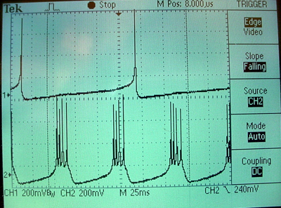
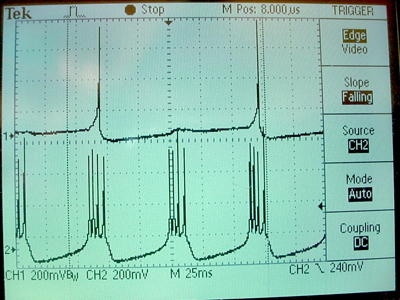
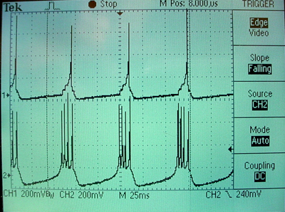
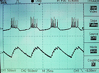
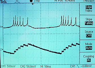
Two scope images show the voltage on the top trace and the membrane recovery variable on the bottom. The traces shown use parameters suitable for a bursting neuron.
The whole project is zipped here.
Two Neurons with modularized construction
The entire neural model, including integrators can be abstracted to a module so that the top-level module has only the neuron instantiations and the interconnections. Interconnections are made by connecting the spike output of one cell to the current input of another. The bias current in this version can be set from the switches and the clock and reset signals are a little cleaner looking. Each of the neurons can have its (binary) spike train brought out to the parallel port.
  // clock divider
	always @ (posedge CLOCK_50)
	begin
		count <= count + 1;
	end
	assign neuronClock = (count==0);

	assign I1 = {2'h0,SW[15:0]} ; //the input bias currents
	assign I2 = {2'h0,SW[15:0]} ;

	assign neuronReset = ~KEY[3]; //the reset pushbutton

	//burster parameters
	assign a1 =  18'sh0_051E ; // 0.02
	assign b =  18'sh0_3333 ; // 0.2
	assign c =  18'sh3_8000 ; // -0.5
	assign d =  18'sh0_051E ; // 0.02
	assign a2 = 18'sh0_041E ; // slightly lower than 0.02

	// define and connect the neurons
	// with inhib cross-connections
	Iz_neuron burst1(v1,s1, a1,b,c,d, (I1-((s2)?18'h0_8000:0)), neuronClock, neuronReset);
	Iz_neuron burst2(v2,s2, a2,b,c,d, (I2-((s1)?18'h0_8000:0)), neuronClock, neuronReset);

	//output spikes to parallel port
	assign GPIO_0[0] = s1;
The neuron module encapsulates all the numerical stuff. Note that the spike output is only one sample (integration step) wide. Each neuron uses 6 multipilers, so the maximum number of neurons that can run in parallel is about 11 For more that that, the system will have to be serialized or simplified. The module produces the voltage variable and a pulse output. The next 4 parameters control the dynamics of the cell. The next parameter is the current input to the cell.
//////////////////////////////////////////////////
//// Izhikevich neuron ///////////////////////////
//////////////////////////////////////////////////
module Iz_neuron(out,spike,a,b,c,d,I,clk,reset);
	output [17:0] out;
	output spike ;
	input signed [17:0] a, b, c, d, I;
	input clk, reset;

	wire signed	[17:0] out;
	reg spike;
	reg  signed	[17:0] v1,u1;
	wire signed	[17:0] u1reset, v1new, u1new, du1;
	wire signed	[17:0] v1xv1, v1xb;
	wire signed	[17:0] p, c14;

	assign p =  18'sh0_4CCC ; // 0.30
	assign c14 = 18'sh1_6666; // 1.4

	assign out = v1;  //copy state var to output

	always @ (posedge clk)
	begin
		if (reset)
		begin
			v1 <= 18'sh3_4CCD ; // -0.7
			u1 <= 18'sh3_CCCD ; // -0.2
			spike <= 0;
		end
		else
		begin
			if ((v1 > p))
			begin
				v1 <= c ;
				u1 <= u1reset ;
				spike <= 1;
			end
			else
			begin
				v1 <= v1new ;
				u1 <= u1new ;
				spike <= 0;
			end
		end
	end

	// dt = 1/16 or 2>>4
	// v1(n+1) = v1(n) + dt*(4*(v1(n)^2) + 5*v1(n) +1.40 - u1(n) + I)
	// but note that what is actually coded is
	// v1(n+1) = v1(n) + (v1(n)^2) + 5/4*v1(n) +1.40/4 - u1(n)/4 + I/4)/4
	signed_mult v1sq(v1xv1, v1, v1);
	assign v1new = v1 + ((v1xv1 + v1+(v1>>>2) + (c14>>>2) - (u1>>>2) + (I>>>2))>>>2);

	// u1(n+1) = u1 + dt*a*(b*v1(n) - u1(n))
	signed_mult bb(v1xb, v1, b);
	signed_mult aa(du1, (v1xb-u1), a);
	assign u1new = u1 + (du1>>>4)  ;
	assign u1reset = u1 + d ;
endmodule
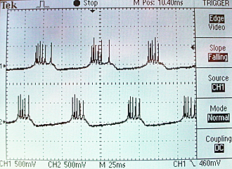
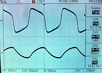
The scope image below showing the voltages of the two neurons was taken with the input current to each of them set to 18'h0_2000.
Optimizing the neuron module and adding a synapse
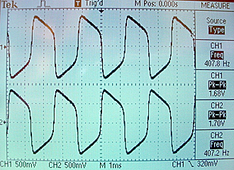
The neural model above uses 6 out of 70 hardware multipliers for each neuron. Looking at the parameter range given in the image from Izhikevich's web site suggests that the a and b parameters don't have to be very accurate for the model to work. The two multiplies by constants were replaced by shifts to approximate the constants within a factor of two. With this change, the number of multipliers drops to two/neuron so that it is possible to put about 35 model neurons on the FPGA. The top-level module was further optimized by introducing a more realistic model of the neuron interconnect (see Ruben Guerrero-Rivera reference below) called a synapse. The new synapse module takes a pulse output from another neuron and uses the impulse (or spike) as a gate to load the initial condition of an exponential decay unit. The scope trace below shows the voltage variable from one neuron, along with the output of the synapse unit driven from the same neuron spike output. You can see that the negative weignt (18'sh3_8000) causes a negative current burst at the time of each action potential.
In the top-level module code shown below, the clock rate has been lowered to the point where individual spikes can be seen on blinking LEDs. Changing the current by flipping switches causes a variety of dynamic behaviors. A switch setting of about 16'h0180 yields alternating bursts. Higher setting cause high-rate synchronous firing.
// clock divider with: reg [15:0] count ;
	always @ (posedge CLOCK_50)
	begin
		count <= count + 1;
	end
	assign neuronClock = (count==0);

	assign I1 = {2'h0,SW[15:0]} ; //the input bias currents
	assign I2 = {2'h0,SW[15:0]}+8 ;

	assign neuronReset = ~KEY[3]; //the reset pushbutton

	//burster parameters
	assign a1 = 6 ;  // 0.016
	assign b =  2 ;  // 0.25
	assign c =  18'sh3_8000 ; // -0.5
	assign d =  18'sh0_051E ; // 0.02
	assign a2 = 6 ;

	// define and connect the neurons
	Iz_neuron neu1(v1,s1, a1,b,c,d, neu1In, neuronClock, neuronReset);
	Iz_neuron neu2(v2,s2, a2,b,c,d, neu2In, neuronClock, neuronReset);
	// with inhibitory cross-connections
	synapse   syn1(neu1In, s2,18'sh3_f000, 1,I1, 0,0, neuronClock, neuronReset);
	synapse   syn2(neu2In, s1,18'sh3_f000, 1,I2, 0,0, neuronClock, neuronReset);

	//output spikes to parallel port
	assign GPIO_0[1] = s1;
	assign GPIO_0[2] = s2;
	// output spikes to the leds
	assign LEDR[1] = s1;
	assign LEDR[2] = s2;
The synapse module is just another numerical integrator which solves the itertative equation
I(n+1) = I(n) - I(n)/16 + spike1*weight1 + spike2*weight2 + spike3*weight3
The divide by 16 yields a reasonable time constant, but could be made a variable.
The synapse module produces a current output variable. The next six parameters are pairs of {spike-input, weight-input} so that each synapse unit has a fan-in of three from other cells.
////////////////////////////////////////
//// Synapse ///////////////////////////
////////////////////////////////////////
// Acts to create an exponentially falling current at the output
// from a spike input and a weight which can be +/-
// up to three spike inputs are defined, each with its own weight
module synapse(out,s1,w1,s2,w2,s3,w3,clk,reset);
	output [17:0] out; 				//the simulated current
	input s1,s2,s3;     			// the action potential inputs
	input signed [17:0] w1,w2,w3;   //weights
	input clk, reset;

	wire signed	[17:0] out;
	reg  signed	[17:0] v1 ;
	wire signed	[17:0] v1new ;

	assign out = v1;  //copy state var to output

	always @ (posedge clk)
	begin
		if (reset) v1 <= 18'sh0; // -0.7
		else v1 <= v1new ;
	end

	// dt = 1/16 or 2>>4 and tau=1
	// v1(n+1) = v1(n) + dt/tau*(-v1(n)+s1*w1+s2*w2+s3*w3)
	assign v1new = v1 + ((-v1)>>>4) + (s1?w1:0)+(s2?w2:0)+(s3?w3:0) ;

endmodule
The optimized neuron module
uses only two hardware multipliers, but makes the a and b parameters settable only to within a power of two. Better resolution could be obtained using another input to set a second shift value.
//////////////////////////////////////////////////
//// Izhikevich neuron ///////////////////////////
//////////////////////////////////////////////////
// Modified to eliminate two of the multiplies
// Since a nd b need not be very precise
// and because 0.02<a<0.2 and 0.1<b<0.3
// Treat the a and b inputs as an index do determine how much to
// shift the intermediate results
// treat the a input as value>>>a with a=1 to 7
// treat the b input as value>>>b with b=1 to 3

module Iz_neuron(out,spike,a,b,c,d,I,clk,reset);
	output [17:0] out; 				//the simulated membrane voltage
	output spike ;     				// the action potential output
	input signed [17:0] c, d, I;   //a,b,c,d set cell dynamics, I is the input current
	input [3:0] a, b ;
	input clk, reset;

	wire signed	[17:0] out;
	reg spike;
	reg  signed	[17:0] v1,u1;
	wire signed	[17:0] u1reset, v1new, u1new, du1;
	wire signed	[17:0] v1xv1, v1xb;
	wire signed	[17:0] p, c14;

	assign p =  18'sh0_4CCC ; // 0.30
	assign c14 = 18'sh1_6666; // 1.4

	assign out = v1;  //copy state var to output

	always @ (posedge clk)
	begin
		if (reset)
		begin
			v1 <= 18'sh3_4CCD ; // -0.7
			u1 <= 18'sh3_CCCD ; // -0.2
			spike <= 0;
		end
		else
		begin
			if ((v1 > p))
			begin
				v1 <= c ;
				u1 <= u1reset ;
				spike <= 1;
			end
			else
			begin
				v1 <= v1new ;
				u1 <= u1new ;
				spike <= 0;
			end
		end
	end

	// dt = 1/16 or 2>>4
	// v1(n+1) = v1(n) + dt*(4*(v1(n)^2) + 5*v1(n) +1.40 - u1(n) + I)
	// but note that what is actually coded is
	// v1(n+1) = v1(n) + (v1(n)^2) + 5/4*v1(n) +1.40/4 - u1(n)/4 + I/4)/4
	signed_mult v1sq(v1xv1, v1, v1);
	assign v1new = v1 + ((v1xv1 + v1+(v1>>>2) + (c14>>>2) - (u1>>>2) + (I>>>2))>>>2);

	// u1(n+1) = u1 + dt*a*(b*v1(n) - u1(n))
	assign v1xb = v1>>>b;         //mult (v1xb, v1, b);
	assign du1 = (v1xb-u1)>>>a ;  //mult (du1, (v1xb-u1), a);
	assign u1new = u1 + (du1>>>4) ;
	assign u1reset = u1 + d ;
endmodule
The
FitzHugh-Nagumo Model with one neuron-like oscillator
The FitzHugh-Naugumo model is a simplified version of the Hodgkin-Huxley model (HH) of nerve action potential production. It is also a variation on the Van der Pol equation. There are two state variables: v is the activation variable and w is the inactivation variable. In HH terms, v is some combination of membrane voltage and the sodium activation, while w is a combination of the sodium inactivation and potassium acitavtion. A matlab code to solve the sysem is shown below. With the constant current shown, the system oscillates. From a numerical point of view, this system is interesting becuase one of the dynamical variables is cubed, which requires some scaling and multipliers.
%FitzHugh-Nagumo Euler version
clear all
clf
dt=.01;
t=0:dt:200;
v = zeros(size(t));
w = zeros(size(t));
v(1) = -0.870;
w(1) = -0.212;
current = .57;
for i=1:length(t)-1
    v(i+1) = v(i) + dt*(v(i) - v(i)^3 - w(i) + current)  ;
    w(i+1) = w(i) + dt*(.08*(v(i) + 0.7 - 0.8*w(i)));
end
plot(t,v)
Converting this to 18 bit fixed point took some scaling and messing with constants. The implemented version with dt=2-6 was
v(i+1) = v(i) + dt*(v(i) - v(i)^3 - w(i) + current)

    w(i+1) = w(i) + dt*(1/16*(v(i) - w(i)))
Notice that constants were rounded to a near power of two. Overflow during summation suggested scaling the variables before adding them. The verilog code in the top-level module was
signed_mult v_2(v2, v, (v>>>1)); // form v-squared/2

    signed_mult v_3(v3, v2, (v>>>1)); // form v-cubed/4

    assign vnew = v + (((v>>>2)-v3-(w>>>2)+(c>>>2))>>>4); //scale vars to match v3 (total shift 6)

    assign wnew = w + (((v>>>1)-(w>>>1)) >>>9); // mult by a factor of 1/16 * dt
(total shift 10)
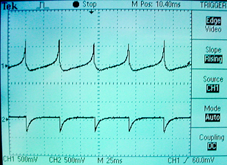
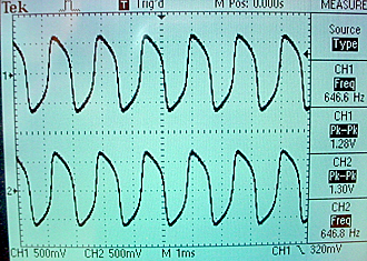
The update rate was scaled to place the waveform in the audio frequency region so that the audio codec could be used for output. A scope display is shown below. The top trace is v and the bottom is w.
The entire project is zipped here.
FitzHugh_Naugumo with two coupled oscillators
Connecting two oscillators together by cross-connecting their activation variables, but with negative sign, causes the oscillators to phase-lock 180 degrees out of phase. There is a lower amplidude metastable state if the starting conditions for the two oscillators are exactly balanced. A current input to the first cell was used to break the symmetry. The main part of the top-level module code is shown below. The cross-coupling occurs because v1/4 is subtracted from the positive feedback for oscillator 2 and v2/4 is subtracted from the positive feedback for oscillator 1.
//analog simulation of FHN system
	always @ (posedge CLOCK_50)
	begin
		count <= count + 1;

		if (KEY[3]==0) //reset
		begin
			v1 <= 18'h3_2148 ; //v1(0) = -0.870;
			w1 <= 18'h3_C9BB ; //w1(0) = -0.212;
			v2 <= 18'h3_2148 ; //v2(0) = -0.870;
			w2 <= 18'h3_C9BB ; //w2(0) = -0.212;
			c <= {SW[15:0],2'h0} ;    // current = 0.35 = 0_5999
			onehalf <= 18'h0_8000;
		end
		else if (count==0)
		begin
			v1 <= v1new ;
			w1 <= w1new ;
			v2 <= v2new ;
			w2 <= w2new ;
		end
	end

	//FitzHugh-Nagumo Equations
	// dt = 2>>6
	//v(i+1) = v(i) + dt*(v(i) - v(i)^3 - w(i) + current)  ;
    //w(i+1) = w(i) + dt*(1/16*(v(i) + 0.5 - 1*w(i)));
	//note that the 0.5 was omitted below

	//cell 1
	signed_mult v_12(v12, v1, (v1>>>1));  	// v-squared/2
	signed_mult v_13(v13, v12, (v1>>>1)); 	// v-cubed/4
	assign v1new = v1 + (((v1>>>2)-v13-(w1>>>2)+(c>>>2)-(v2>>>4))>>>4); //scale other vars to match v3
	assign w1new = w1 + (((v1>>>1)-(w1>>>1)) >>>9); // mult by a factor of 1/16 * dt
	//cell 2
	signed_mult v_22(v22, v2, (v2>>>1));  	// v-squared/2
	signed_mult v_23(v23, v22, (v2>>>1)); 	// v-cubed/4
	assign v2new = v2 + (((v2>>>2)-v23-(w2>>>2)-(v1>>>4))>>>4); //scale other vars to match v3
	assign w2new = w2 + (((v2>>>1)-(w2>>>1)) >>>9); // mult by a factor of 1/16 * dt
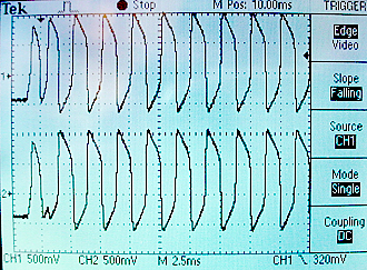
The 180 degree phase-lock state is shown below. Biologically, this corresponds to reciprocal inhibitory synapses between the two oscillators forcing them into alternation.
The metastable in-phase state is shown below. Notice that the amplitude is smaller because each oscillator is inhibiting the other. The next figure shows the shift from in-phase to 180 phase for a very small difference in starting conditions. Note that both oscillators rise in phase on the first cycle, but by the third cycle to two are 180 phase-locked. The flat trace to the left of the trigger represents the reset state.
The whole project is zipped here.
References
- Ruben Guerrero-Rivera, et al, Programmable Logic Construction Kits for Hyper-Real-Time Neuronal Modeling, Neural Computation, Volume 18 , Issue 11 (November 2006) Pages: 2651 - 2679
- Eugene M. Izhikevich , Simple Model of Spiking Neurons,
IEEE Transactions on Neural Networks (2003) 14:1569- 1572