
ECE 576 – Final Project
Donn Kim (ddk26)
Antonio Dorset (acd32)
Contents
The goal of this final project was to create a sound spatialization system. A sound spatialization system makes a sound source appear to originate from different points in space when listened to using headphones. For example, this system can make the music coming from a normal music player sound like it is coming from some point in space to the listener’s right, simply through signal processing. The main components of this project were the Altera DE2 development board, Quartus II web edition, the NIOS II IDE, and a high quality set of earphones. This system could vary the azimuth position of the sound source from 0 to 360 degrees in 5-degree increments. The apparent elevation of the sound source could also be varied between -20 degrees, 0 degrees, and +20 degrees anywhere along the azimuth positions. Fig. 1 shows the definition of azimuth and elevation in the context of this system.
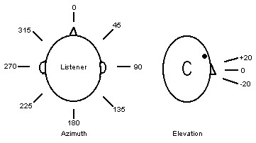
Figure 1: Definition of elevation and azimuth
There were two ways to choose the desired azimuth: using switches SW[0] to SW[6] to enter a binary number between 0 and 71 (which when multiplied by 5 would represent azimuths from 0 to 355), or using the four keys – KEY[0], KEY[1], KEY[2], and KEY[3]. KEY[3] incremented the azimuth by 5 degrees, KEY[2] decremented the azimuth by 5 degrees, KEY[1] incremented the azimuth by 90 degrees, and KEY[0] decremented the azimuth by 90 degrees. The elevation was chosen using switches SW[8] and SW[9]. When SW[8] was low, an elevation of 0 was chosen. When SW[8] was high, the elevation could be chosen by setting SW[9] high (elevation of +20) or setting SW[9] low (elevation of -20).
II. Design and Testing Methods:
Humans use a variety of methods to determine where a sound is coming from. The simplest are interaural time differences (ITDs) and interaural level differences (ILDs). Interaural time differences represent the difference in arrival times of sound waves from a sound source to the left and right ears. For example, sounds waves from a sound source located at an azimuth of 45 degrees will reach the right ear earlier than the left ear. In addition, the sound waves that reach the left ear will be slightly attenuated compared to the left ear because of shadowing effects from the listener’s head – this represents interaural level differences.
It is possible to create a rudimentary sound spatialization system based on ITDs and ILDs alone. However, there are certain issues that arise when using only these two localization cues. First, ILDs are not linear with respect to frequency. This is because sound waves with frequencies of about 1500 Hz have wavelengths that are on the order of the diameter of the human head. Thus, frequencies lower than 1500 Hz are not attenuated much by the head at all, while frequencies above 1500 Hz are attenuated a great deal. Thus, ILDs are the dominant cues at high frequencies. Additionally, above 1500 Hz, ITDs are greater than one period of the incoming wave, which leads to aliasing errors. Thus, ITDs are the dominant cues at lower frequencies.
The problem is exacerbated once elevations are taken into account. Very often, sounds from sources at elevations that are similar to each other will have the same ITDs and ILDs, leading to a so called “cone-of-confusion” in which the sound source cannot be determined accurately. Another problem is that a sound signal that is processed using only ITDs and ILDs appears to originate from inside the listener’s head, which is a disturbing effect.
Because humans have become very good at localizing sound sources, it is apparent that there are other mechanisms used to provide cues besides ITDs and ILDs. It is believed that incoming sound waves have their spectral content altered by reflections from the listener’s head, shoulders, and torso, which the human brain processes to extract more localization cues. This filtering effect is referred to as the Head Related Transfer Function (HRTF). Since every person’s body dimensions and ear shapes are different, every person has a unique set of HRTFs that the brain is tuned for. The HRTFs contain both ITD and ILD cues, as well as the spectral filtering effects.
Luckily for us, the Media Lab at MIT has already made a multitude of HRTF measurements using a dummy named KEMAR. KEMAR is a faithful representation of a human torso, head, and ear canal. Different ears can be attached to create different responses. A tiny microphone was placed deep inside the ear canal to make recordings as the sound source was moved around. The resulting information was processed to create the HRTFs.
We used the diffuse field equalized HRTFs from the MIT Media Lab website after consulting with Bill Gardner, who took the measurements. This was a reduced data set of 128-point, 16-bit signed integer HRTFs derived from the left ear KEMAR responses. For example, the left ear response for an azimuth of 90 degrees was derived from the 90 degree response of the left ear KEMAR data set, while the right ear response for the same azimuth was derived from the 270 degree left ear KEMAR data set. Because there was so much data to process (128 HRTF coefficients for each ear for each of the 72 azimuth increments, at three different elevations), a Matlab script was written to manipulate the data, as shown in Fig. 2.
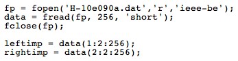
Figure 2: Example Matlab script to process data
The data for all of the azimuth increments was put into 2D arrays for each of the three possible elevations. Each of these arrays was 72x128, representing 128 HRTF coefficients for each of the 72 possible azimuth increments.
There were three main components of this lab – Verilog code for the hardware, a NiosII/e CPU, and C code for the CPU to run. All three files were necessary to provide the hardware and processing support needed to handle the large number of coefficients and constants needed for each ear at each elevation and azimuth.
The Verilog code was spread among three main files: DE2_Default, Audio_ADC_DAC, and I2C_AV_config. DE2_Default wires together the reset generator, PLL audio clock generator, I2C codec configuration module, and the audio module. This file also determined the azimuth angle and elevation angle. When switch SW[17] was low, switches SW[6] to SW[0] were interpreted as the azimuth angle. Because 7-bits could represent numbers greater than 71, code was written to make the maximum value of the azimuth angle 71, even if a higher number was selected. When switch SW[17] was high, buttons KEY[3] to KEY[0] selected the azimuth angle. KEY[3] increased the azimuth angle by 5 degrees, KEY[2] decreased the azimuth angle by 5 degrees, KEY[1] increased the azimuth angle by 90 degrees, and KEY[0] decreased the azimuth angle by 90 degrees. Instead of having the angles display a value greater than 360 degrees code was written to cause the azimuth angle to wrap around if the current angle was increased above 355 degrees or decreased below 0 degrees so that the operator will know the direction the sound is coming from in a 360 degree span around his/her head. For example, if the current azimuth angle was 290 degrees and KEY[1] was pressed to increase the azimuth angle by 90 degrees, the new azimuth angle was 20 degrees (i.e. 290 o + 90 o).
The I2C codec configuration module configured the audio codec to our specifications. Because the KEMAR HRTFs were sampled at 44.1 kHz, our input and output sample rate also had to be set to 44.1 kHz. We chose to use the line-in input as opposed to the microphone input so that we could have control over the gain of the input. The line-out output was used because the DE2 board did not have headphone outputs, though the audio codec supported it. The specifics of the configuration registers can be determined by downloading the data sheet for the Wolfson Microelectronics WM8731 audio codec. The values of our configuration registers are shown in Fig. 3. Note that one word of dummy data must be sent across the I2C interface before the first actual setup parameter to allow the audio codec to initialize.
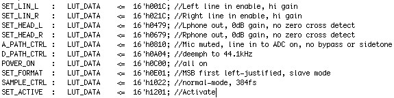
Figure 3: Audio codec configuration
The Audio_ADC_DAC is the main file for this project. The bulk of this file was occupied by the state machine, which acts as a finite impulse response filter. For each given azimuth and elevation, the current input and the past 127 inputs have to be convolved with the 128 HRTF coefficients. This is done for each ear. This is represented in Fig. 4.
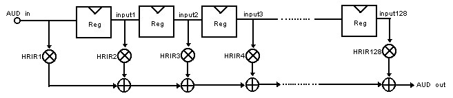
Figure 4: 128-point finite impulse response filter
Because there is too much data and it would require too many multipliers to do all of the multiplications at once, a state machine was used to do only one multiply and accumulate at a time. Once all 128 multiply and accumulates were done, the result was outputted to the audio codec.
The HRTF coefficients were stored in separate m4k blocks for each ear. The ROM module was based on the code on the DE2 hardware page, as shown in Fig. 5.
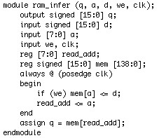
Figure 5: ROM module
In each step of the state machine, the memory address to be accessed was sequentially incremented, because the HRTFs were stored in order. It takes two state machine steps for the HRTF coefficient to be read from memory, at which point the HRTF coefficient for each ear was sent to separate multiplier modules along with the registered value of the input. The input was sent to both the left and right multipliers because only one channel of the input was used. A separate module was used for the multiply function because it greatly reduced the compilation time. The result from the multiplier was ready after two state machine steps, at which time it was accumulated. Fig. 6 shows the code that accomplished this, and Fig. 7 is a pictorial representation of the state machine. At startup, the state machine takes 132 steps because of the additional cycles needed to read from memory and get the result from the multiplier module. However, once the state machine ran it took 128 steps because memory was being read at every step. In order to have audio with no artifacts, static, or other anomalies, the state machine has to multiply and accumulate all 128 inputs before the DAC is sampled to be output. This was easily accomplished because the state machine was run at a clock rate of 50 MHz, compared to the sample rate of 44.1 kHz.
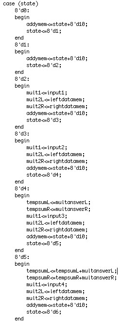
Figure 6: Partial state machine code
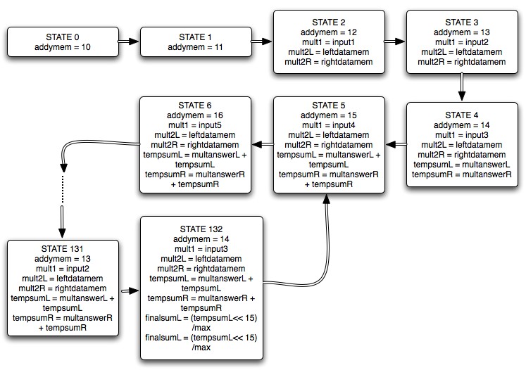
Figure 7: Pictorial representation of state machine
Because the HRTF coefficients did not add up to one, the accumulated value had to be normalized before being outputted. Failing to do so resulted in an output that was garbled and unusable. To get around this issue, the final accumulated value was checked against a maximum value that was saved. If the accumulated value was larger than the previous maximum value, the maximum value was updated. The final accumulated value was divided by the maximum value, then shifted to the left by 15 places because the DAC input was a 16-bit signed integer. When testing, we found that the output creating a clicking noise, implying that the resulting value was overflowing. This was remedied by adding 35 to the maximum value that was saved thus preventing this overflow. We also found out that when there was no input, there was still a low level distorted sound being outputted (i.e. noise). This was solved by setting any input that was between -8 and 8 to 0 thus changing the threshold value for the input signal and eliminating random noise. It was important to make the accumulator register at least 39 bits wide. This was because both the input and the HRTFs were 16 bit values, leading to a maximum value that was 32 bits wide. Also, since there were 128 values being accumulated, the maximum possible value for the accumulation was 39 bits.
The Audio_ADC_DAC file was based off of the example on the DE2 hardware page. The only other changes that had to be made were to change the reference clock and the sample rate. The sample rate was set to 44.1 kHz because that was the frequency at which the HRTFs were sampled. The reference clock was changed to 16.9344 MHz because this is what the audio codec data sheet specified for a sample rate of 44.1 kHz.
The next large piece of this project was the CPU. A NiosII/e CPU was used because we did not need the features of the higher level versions. The CPU was created using the document called “Introduction to the Altera SOPC Builder Using Verilog Design.” Besides adding the CPU, JTAG UART protocol, and the on-board memory, the following input and output ports were created (Fig. 8):
a) addycpu: 8-bit output to represent the memory address to write to
b) ledg: 8-bit output to aid in debugging by using the green LEDs
c) leftdatacpu: 16-bit signed output representing the HRTFs to be written to memory for
the left ear
d) rightdatacpu: 16-bit signed output representing the HRTFs to be written to memory for
the right ear
e) sw: 8-bit volatile input representing the desired azimuth angle
f) sw8: 1-bit input representing whether a flat sound source was desired
g) sw9: 1-bit input representing whether an elevation of -20 or +20 degrees was desired
h) we: 1-bit output that determined whether or not the ROM that was instantiated in
Audio_ADC_DAC was written to
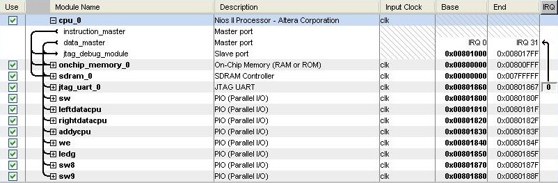
Figure 8: Screenshot of SOPC Builder
Since there was so much data to be stored, we decided to use the SDRAM that was present on the DE2 board. SDRAM was instantiated using the document called “Using the SDRAM Memory on Altera’s DE2 Board with Verilog Design.” This required the creation of a phase locked loop, because of the requisite set-up time of the SDRAM chips. The PLL was instantiated in the DE2_Default file and advanced the clock being fed to the SDRAM chips by 3 ns in relation to the 50 MHz clock for the rest of the system. Because SDRAM was used, a few more parameters had to be passed to the CPU when it was instantiated in Audio_ADC_DAC. These parameters can be found in the nios_system.v file.
The C code less complex than the Verilog code. The majority of this file was taken up by the HRTF data. Whenever the azimuth of elevation angle was changed, the write enable was asserted to write the new HRTF values to the ROMs for the left and right ears. A loop then outputted the data from one of the three sets of data (elevations of -20, 0 and +20). The address was incremented at the same time. For example, if switch SW[8] was low, the 128 HRTFs from the appropriate row of righthrir and lefthrir would be outputted. If SW[8] was high and SW[9] was high, the HRTFs from righthrirpos20 and lefthrirpos20 would be outputted. If SW[8] was high and SW[9] was low, the HRTFs from righthrirneg20 and lefthrirneg20 would be outputted.
The biggest challenges that we faced were bad design and long compile times. In our first design, we did not use a CPU and instead placed all of the HRTFs into M4K blocks. This design took over an hour to compile, at which point the compiler informed us that the design would not fit. This problem was resolved using a CPU with SDRAM. The second bad design was having the multiplies occur within the individual states of the state machine. Once again, the compile times were extremely long and the compiler informed us again that the design would not fit. This was remedied by having a separate module take care of the multiply function, with each state sending the multiplier module the numbers to be multiplied. This reduced our compile times to about 25 minutes. The compile time was further reduced to about 10 minutes by turning on the Smart Fit feature in the Quartus II program.
The final challenge was getting a clean output from the audio codec. The first revision of the working project had an output that contained static and would produce pops every so often. The pops were fixed by changing the normalization values so that the accumulated number would not overflow. The static was fixed by setting low signals (-8 to 8 in a range of -32768 to 32767) to 0.
Our sound specialization system performed as designed. The system was able to take a sound source as an input (i.e. from a microphone or music source like an Ipod), and output the sound at different spatial angles from the perspective of the listener. For the user listening to the sound, changing the angle of the system made the sounds source appear as if it was changing in space along a 360 degree azimuth and a -20 to +20 degree elevation. Music was inputted into the DE2 board’s line-in where it was processed by the hardware (i.e. Verilog code). The audio codec sampled the input music at 44.1 kHz. The switches and determined what angle the sound should appeared to be coming from. With an 72 different azimuth positions (i.e. 360 degrees in 5 degree increments) and 3 different elevation positions (i.e. -20, 0 and +20 degrees), our system provided 72 x 3 = 146 possible positions in space in which to position a sound. Since each of the 72 possible azimuth positions consisted of 256 different coefficients (i.e. 128 for the left ear and 128 for the right ear) the NiosII/e CPU provided the processing power to handle the constant loading of these coefficients. When a position is chosen the CPU loaded the 256 different coefficients in M4K blocks that the Verilog code would use to perform a convolution with the sampled sound input to produce the desired sound specialized output. Even though our system worked as designed, it worked differently for every person that used it. This is because the coefficients for the Head Related Transfer Function were calculated based on the shape of the KEMAR dummy head and ear canal. Therefore, whenever anyone with dimensions much different from those of the KEMAR dummy use the system, their perception of the sound in space is slightly different. This became apparent during our demonstration of the system.