ECE5760 Final Project:
Capital Letter Recognition with Harris Corner

Rationale and Sources

In computer vision, the Harris Corner feature plays an important role as early steps in many detection algorithms. However, the overall calculation involves multiple matrix summation, reduction and multiplication which makes it relatively time consuming to implement on a CPU based implementation. One way to speed up the process is to design a hardware accelerator for this specific algorithm since most of the calculations can be parallelized as well as pipelined. The Field Programmable Gate Array (FPGA) is a piece of hardware with great flexibility, therefore it is a good tool to serve our purpose. There are some previous works related to implementing the Harris Corner algorithm based on FPGAs. The Wong’s team implemented a real-time Harris Corner algorithm for a resolution of 640*480 with a window size of 5 by 5 on the Avnet Zedboard [1]. The Kasnakoglu’s group implemented a pipelined FPGA architecture to detect corners in colored stereo images using the Harris Corner algorithm based on a Xilinx FPGA board [2]. We found an interesting implementation of this algorithm with Gaussian smoothing filter integrated on Matlab, which we thought can improve efficiency of FPGA implementation [3].

System’s principle & background math

Harris Corner algorithm

The Harris Corner algorithm will take a small windows of the image (e.g. 3 by 3 pixels in our case) and determine whether the center of the pixel is a corner or not based on the response(R) as shown in equation (1):

$$R = Det(M) - k * Trace (M)^2 $$

The Structure Tensor matrix M is depending on the derivative of the image along the x and y axis. Assume I (x,y) is the intensity of the pixel at the image at index (x, y) as shown in Figure 1. W is a filter whose coefficients are determined by Gaussian distribution. The result will be the sum of the dot products for the window and matrix M at each center pixel. The value of k is a constant around 0.04-0.06.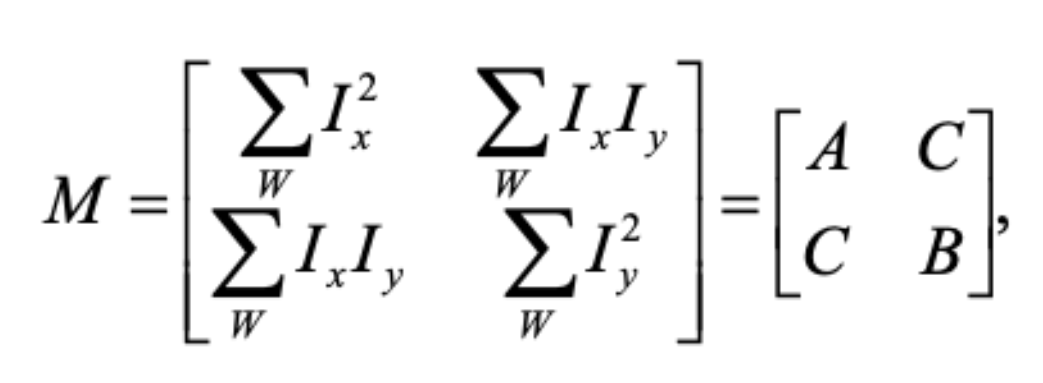

Figure 1. The Structure Tensor matrix M in harris corner.

As a result, the overall calculation will break down into several pieces as shown in equation (2):

$$R = Det(M) - k * Trace (M)^2 = AB – C^2 – k * (A+B)^2 $$

Once we have the response matrix, we can set up a threshold value to indicate whether there is a corner. The value of threshold is an experimental value which we choose 0.1. In order to select the most likely corner in a pixel, we use a technique called “non-maximum suppression” which we shift a 3 by 3 window along the “candidates” of corners (the response matrix after threshold) and pick only the maximum response value within the window and clears all the remaining candidates.

Recognition algorithm

We used two different statistical analysis approaches for our recognition system. The first approach is the probability density function. The probability density function can provide a relative likelihood that the value of the random variable would equal that sample. The probability value is given by the integral of this variable's PDF over that range and the given sigma's value. We will use the normal PDF equation (3) to determine both image’s similarity.

$$ f(x; \mu,\sigma^2) = \frac{1}{\sigma\sqrt{2\pi}}e^{-\frac{1}{2}(\frac{x-\mu}{\sigma})^2} $$

The second approach is the Kullback–Leibler divergence. It is the sum of the equation (4):

$$D_KL(f || g) = {\sum_{x \in \chi}}f(x)log(\frac{f(x)}{g(x)})$$

Since we need to compare the corner’s distribution between the testing image and the training image, the K-L divergence can show the similarity between the distribution defined by g and the reference distribution defined by f. If the sum is lower, then the similarity between two images would be higher.

Logical structure

Our design can be categorized into two parts: hardware and software. Hardware implements the Harris corner detection algorithm and software is used for preprocessing images and Alphabet letter inference. The detailed Qsys setup is shown in Figure 3. The VGA SRAM, VGA_Subsystem and VGA on chip buffer are connected in order to draw on the computer screen directly from the FPGA. The onship SRAM is a communication buffer to exchange data between the HPS and FPGA. Since we do not have physical access to the lab this semester, we send the reset signal to the FPGA through a PIO called “pio_rst” which is on the light weight axi bus. Once the user hits ‘R’ or ‘r’ on the keyboard, the program will send a reset signal and the FPGA will start computing the Harris Corners. The program will also record the computation time and display in the console.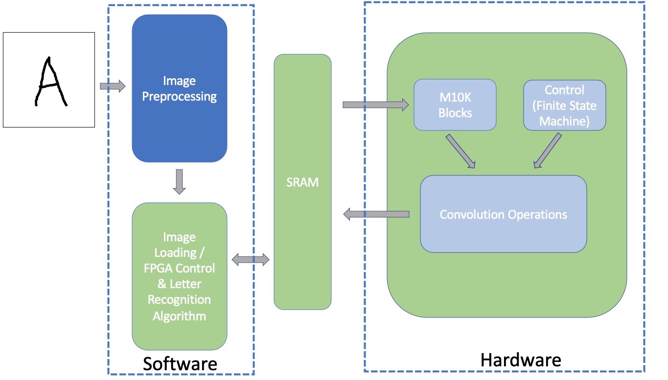

Figure 2. The block diagram of the system scheme.

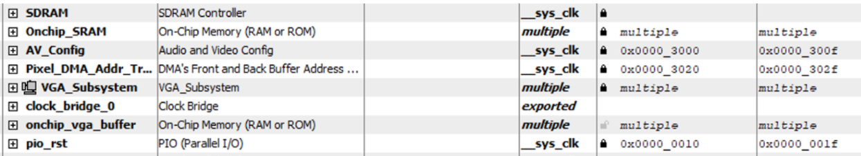
Figure 3. The Qsys setup.

Hardware/software trade offs

One of the tradeoffs we made is that we originally store all the temporary results during the calculation in register files so that we can access them in parallel which will lead to a one cycle latency for calculating the convolutions. However, the drawbacks of this implementation is that the logic to index the pixels are very complicated since we have to select 9 (3 by 3) pixels every time for convolution. It can pass all the simulation results but it needs way too much logic (LUTs) to implement the selection logic based on the synthesized results which will discuss in detail in a later section. In order to solve this issue, we store all the temporary results into M10k blocks (SRAMs) to save the usage of logic because we can read or write the results from the memory block based on the read or write address. However, the price we have to pay is we need nine cycles instead of one to read out all the pixels for convolution each time. One potential improvement we could do is to use a line buffer to speed-up the process but it will introduce additional hardwares. The other tradeoff in our hardware design is we divide the response by 16 by shifting right each partial sum accordingly in equation 2. The reason we introduce these additional shift operations is to avoid overflow during calculation. It is harmless even though we lose some precision during the calculation because we only care about the response value bigger than the threshold and the smaller numbers are ignored anyway. In addition, the shift operations are relatively cheap so they just introduce negligible overhead. Another compromise we made during the design is to give up the pipelined structure due to the limited DSP resources on the board. If there are more DSP blocks available on the board, we could parallel the computation and at the same time pipelined the overall structure to further increase the throughput. Unfortunately, there are only 87 DSP blocks on the board and we have to reuse some of the multiplier during convolution which makes pipelined structure infeasible to implement.

Hardware Design

Image storage

We first implement a Matlab version of the harris corner which we use for verification. Based on the value range of all numbers throughout the calculation, we decide to use a 6.21 floating point representation for our numbers which can not only avoid an overflow issue as well as keep the maximum possible accuracy. Another reason to choose this floating point representation is to limit the usage of the DSP blocks on the FPGA since each DSP block can be used as a 27 by 27 multiplier. The images are passed from HPS to FPGA through SRAMs which can avoid re-run the synthesize each time. In order to perform convolution successfully over a 3 by 3 window, we append a zero(zero-padding) around the image which leads to an initialization of 1024 blocks in the SRAM. The storage of the image was formed into an 1D array by concatenating row by row of pixels, and therefore, the addresses of the memory locations are indexed from upper-left as zero and bottom-right as 1023. For simplicity of operating pointers, we initialize these numbers into integer data type which is 32 bits and drop the most significant 5 bits when it is passed to the FPGA.

Computation

The core of implementing the Harris Corner detection algorithm on the FPGA is to construct the structure tensor matrix M. We have divided the workflow into the following steps to achieve this:

1. Calculating spatial derivatives of the input image —Ix and Iy
2. Calculating the products of derivatives for each pixel of the image —Ix², Iy², and Ix*Iy
3. Calculating the sums of the products from step 2 for each pixel in window W — Sx, Sy, and Sxy
4. Applying the equation 2 to compute the Harris response value — R

It is always a good idea to filter out the noises on an image before it gets processed. We employed a 3 by 3 2D Gaussian filter with a σ of 1 as the Gaussian filter is symmetric and separeable. Therefore, the operations of flipping kernels for performing convolution can be saved and the spatial derivatives of the image can be computed by convolving the image with the partial derivatives of the Gaussian equation with respect to x and y as kernels, respectively. The partial derivatives can be calculated beforehand via Matlab and stored in registers on the FPGA. Once the spatial derivatives are computed, the corresponding products can be computed within the same clock cycle. The benefits of using Gaussian kernels can also be embodied in the way the sums of the products are computed. Again, we only need to convolve the products of derivatives with the Gaussian kernel as window function parallelly to fast compute sums of the products of the derivatives. By conducting this approach, the structure tensor can be constructed in a hardware-accelerated fashion. In addition, the computations running on FPGA have been simplified into repetition of convolutions, resulting in amelioration of complexity and enhancement of parallel computation.

Convolution

The major operations running on the FPGA are 2D discrete convolutions, and most of them can operate parallelly. Ix and Iy can be computed parallelly as they require the same image patch that is formed by shifting a 3 by 3 window left-to-right then up-to-bottom across the original image. Squaring and multiplying the spatial derivatives at each pixel yields the products, which are written to M10K blocks and are going to be fed as inputs to the next convolution operations. Sx, Sy, and Sxy can be computed parallelly as they require the same kernel Gxy. Convolutions in our case can be implemented as computing inner products of two 3 by 3 matrices. The Figure 4 illustrates this process. We used 9 registers to temporarily store the image patch, generated 9 signed multipliers for calculating the products and then fed the results to adder trees in order to make sure the synthesis tool can handle the timing requirement of hardware. Since the pixels are stored as an array of 27-bit binaries in the memory, finding the memory locations of the corresponding pixels of the changing image patch as the kernel shifts is very important. In addition, it takes 2 clock cycles to read from M10K blocks and the way schedule timing must be under consideration. We implemented a specific finite state machine to control the addresses for pipeline reading memories.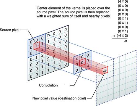

Figure 4. An Example of Computing 2D Convolution. [4]

Software Design

Matlab training/testing simulation

Before we designed the Harris Corner algorithm on the verilog, we wrote a Matlab script to test our ideas and prepared it for the later debugging. The Harris Corner algorithm was the same concept that was mentioned in the previous section. The program will convert the input images to a grayscale image and then make it become binarized. After that, the program will determine the object’s boundaries based on the pixel’s value. It will find the first column/row and the last column/row that contains the non-zero value to identify the object's location and add 20 additional rows and columns along with the bounding box. Then, we used the built-in function to resize the image to 30x30 arrays and convoluted the image with the 3x3 Gaussian filter matrix for the x and y directions. After that, the program will compute the products of the derivatives at every pixel and the sum of the products of the derivative of each pixel. Last, it will compute the response of the detector at each pixel by using the equation (1) that shows above. We used the process to train 45 sets of 26 letters (1170 images in total) for being our training database. Those handwritten images were written by our friends. The flowchart of the process is shown in Figure 5.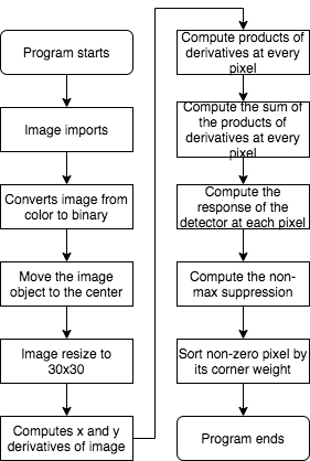

Figure 5. The flowchart of the Harris Corner detection in Matlab.

Once we finished the Harris Corner program, we designed our own letter recognition system which was similar to the K-Nearest Neighbors Algorithm (KNN). The KNN algorithm uses ‘feature similarity’ to predict the values of any new data points. This means that the new point is assigned a value based on how closely it resembles the points in the training set. In our design, we used the normal density distribution and Kullback–Leibler divergence to determine the similarity between the testing set and the training set. Since the number of coordinates for each image was different, the program will find the smaller number from the training set and the testing set. After that, the program will sort the testing coordinates by comparing the distance between the training set in order to make the result better. For example, there were three coordinates in both the training set and testing set, which were {[1,1],[3,3],[5,5]} and {[3,4],[5,4],[2,1]} respectively. Then, the testing coordinates will be sorted into {[2,1],[3,4],[5,4]} based on the distance for the corresponding coordinates of the training set. After that, the program will compute the normal PDF and KL divergence for x coordinates and y coordinates. For the normal PDF, we stored two types of data in the storage list. The first type was the sum of the product of the X and Y PDF. In this type, we treated each coordinate point individually. The second type was the product of the sum X PDF and the sum Y PDF. In this type, we treated the coordinates all together as a single object. So, the storage will store these three different values into three different columns. When all the training images are compared with the testing set, the program will start to count the most possible index for each set by finding the maximum PDF and the minimum KL. (Note: each set has 26 data. Each data has three columns of values) Therefore, it will return a 26x3 array that identifies the possible chances for each letter. The program then starts voting from these values by finding the index (1-26) of the maximum values in each column. If there are two columns that have the same index, the program will pick the corresponding letter as the final answer. If there are no columns that have the same index, the program will pick the index that has the largest count to be the final answer. The flowchart of the program is shown in Figure 6.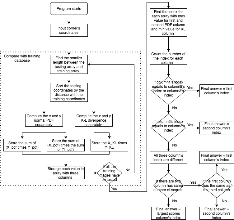

Figure 6. The flowchart of the letter recognition in Matlab.

HPS program

The purpose of the HPS program was to send the image array to the FPGA and predict the possible letter from the corner result that was computed by the FPGA. Therefore, the program was designed to ask the user to enter the letter of the image and the image’s array through the command console. Then, a for loop array will send each element of the array through each SRAM address. Since the array size was 32x32 (a 30x30 image with two additional boundaries for the convolution) and a finished flag needs to be stored in the SRAM addresses, we set the SRAM address to 11 bits in order to satisfy the number requirement. When the program finished storing the pixel values to the SRAM, the HPS would ask the user to reset the PIO port. Once the pio port was rest, the finished flag would be set to one, which was used to tell the FPGA that all the data was ready and the computation could be proceeded. The HPS side would wait until the FPGA wrote the finished flag to zero. After the HPS received the message, the computation time would be recorded and displayed on the VGA screen. In the meanwhile,the program would start computing the non-max suppression. The purpose of non-max suppression was to select the best bounding box for an object and reject or “suppress” all other bounding boxes, so we could have many clear corners of the image. Then, the program would record the non-zero pixels’ coordinates and return a 2D array with x and y coordinates, so the array can be input into the letter recognition system that was the same as the program in Matlab. After the prediction process, the program would compare the answer with the initial user input to determine whether the recognition was correct or not. If the prediction was correct, the VGA would show a green box with a “Bingo” message. On the other hand, the VGA would show a red box with a “Fail” message if the program got a wrong answer. The process is shown in Figure 7.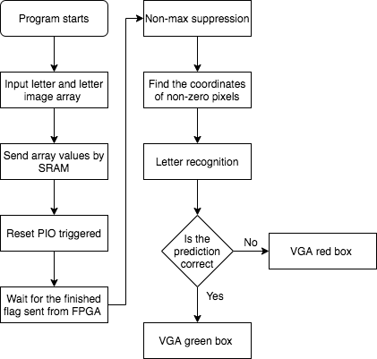

Figure 7. The flowchart of the HPS program.

In the original design, we used the registers to store each pixel instead of using the M10K blocks. Although we could get a correct result from the Multisim simulation, we got the error messages that show in Figure 8 while compiling on the board. After discussing with the instructors, we found out that the registers’ array indexing requires more Look-Up Tables (LUTs) for selecting logics, so we decided to store images directly through the M10K memory blocks. After the change, the logic utilization was reduced from 3464% to only 16%, which shows in Figure 9. Although the state machine became more complicated in order to synchronize the M10K memory, the M10K blocks brought huge benefits to reduce the usage of the board resources.

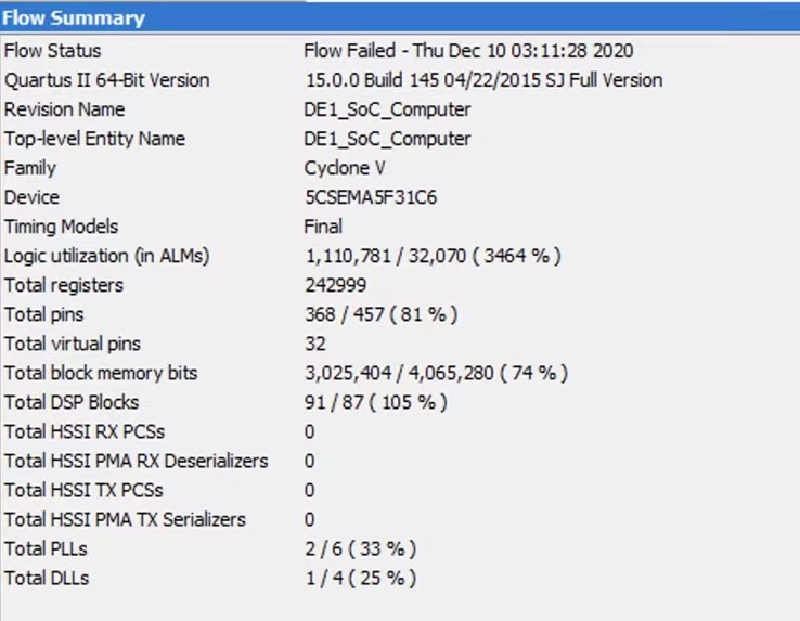
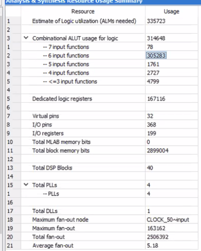
Figure 8. Error messages while compiling Verilog.

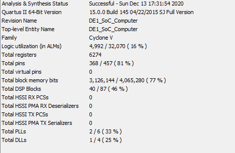
Figure 9. The compiling report after using M10K blocks.

Before implementing the letter recognition algorithm on the board, we used Matlab to do the simulation for 260 images (each letter has 10 images). The results are shown in Figure 10. We found that the percentage of the letter can be successfully predicted by one of the three methods was 63.08%, but after the voting process, the percentage became 50%. We noticed that the accuracy of the prediction was dependent on the voting threshold and 50% was the perfect accuracy we got from the experiments. If we had more time, we could optimize the voting process or use other machine learning approaches to determine the capital letter.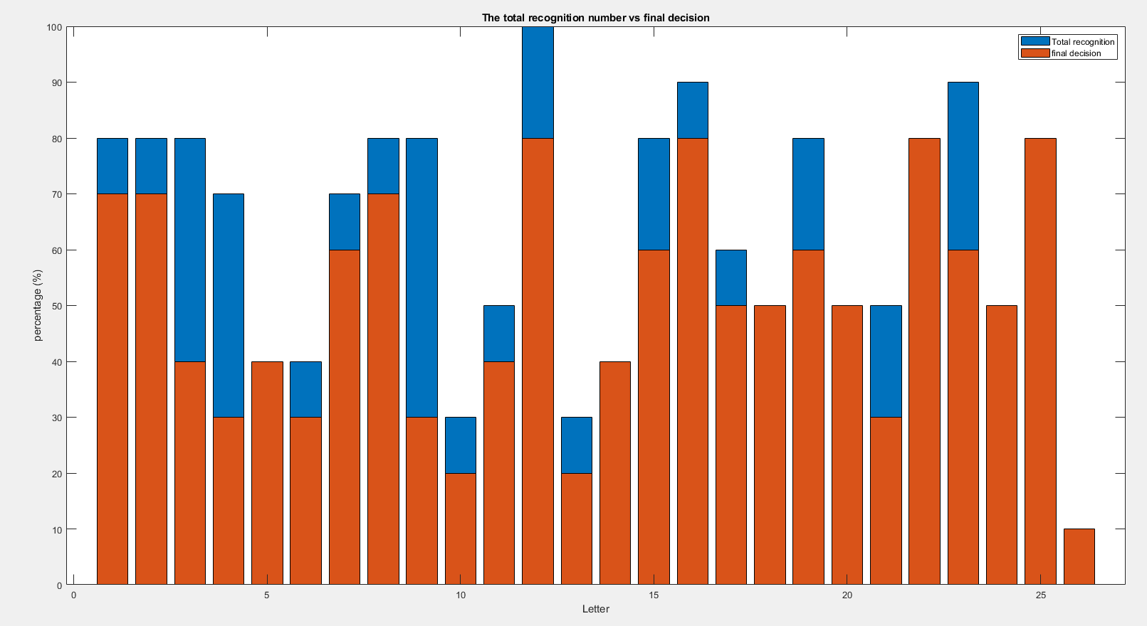

Figure 10. Letter recognition accuracy.

After we tested the letter recognition system, we developed a Matlab application that was able to output the image array, so the user can directly input the array into the command line. The reason we decided not to use the HPS to do the image processing was that we thought the process of uploading images was not convenient to demonstrate or friendly to test multiple images. With this app, the user would just need to import the image from the computer and enter the array into the command line. Besides, this application was a standalone app, so it could be installed on every computer, which was much more reliable. The application’s interface is shown in Figure 11.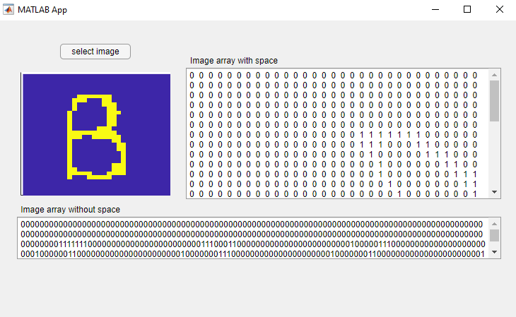

Figure 11. Matlab application.

Once we finished all the preparations, we tested our system with different images and the results are shown in Figure 12. We could see when the letter was predicted right, the green box and a smile face would appear. However, if the prediction went wrong, the red box with a sad face will show and the system will tell the user which letter it thought to be. We found the accuracy performance was not good enough as the simulation due to the precision. The reason was that we used a 6.21 fixed point on the FPGA, so the precision of the result can only be 8 decimal digits, but the simulation can have 16 decimal digits accuracy.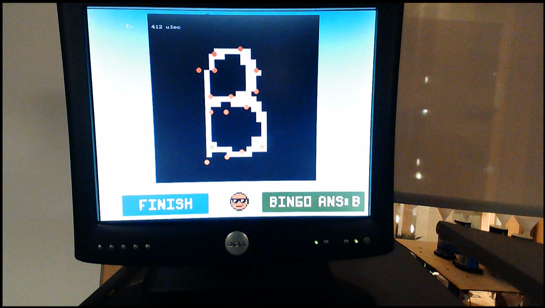

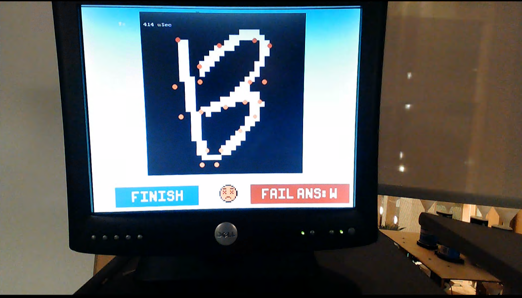
Figure 12. Image recognition succeeds. (left) Image recognition failed. (right)

In addition, our system can not only test the binary image but also a grayscale image because we used the Gaussian filter to calculate the convolution, so the array would be symmetrical. We tested Piet Cornelies Mondrian's famous drawing in Figure 13 (left) and converted it to a grayscale image array. After processing the image in our system, the result is shown in Figure 13 (middle). Although we cannot display the grayscale image on the FPGA, we can show the corner coordinates of the image that shows. Then, we compared it with the Matlab simulation in Figure 13 (right) and found that the coordinates distribution was pretty similar, so we believed that our system worked properly for both binary and grayscale images.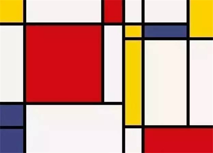

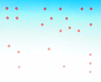
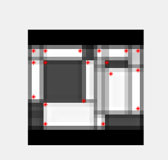
Figure 13. Gray image’s corners detection displayed on VGA.

Last, we tested the computation time of the system. The FPGA computation time to find the Harris corner array was about 0.5 milliseconds, which was faster than the Matlab computation time 1.629 milliseconds. One thing worth mentioning is that these numbers are not fairly “compared” since they have a huge difference in clock frequency. The Matlab is running on a processor of 3.6 GHz which is about 586,440 cycles while the FPGA operates on a 50 MHz clock which is about 25,000 clock cycles. Therefore the FPGA has a speed-up of 23x for finding the harris corner. Besides, the total computation time that included the letter recognition was 7222.224 milliseconds on the board and the total computation time on Matlab was 133.18 milliseconds. These times were both calculated in a real-time. The result matched our expectations because the HPS required more for loop arrays to sort and find the maximum/minimum value of the lists. Matlab has lots of built-in functions that could do this process without using for loop, so the time can be faster. The output results are shown in Figure 14.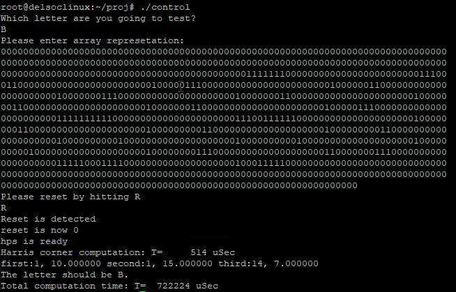

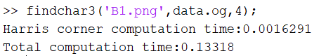
Figure 14. FPGA and HPS result output (left). Matlab computation output (right).

We also run the power anysize on a tool provided by Quartas and the result is shown in Figure 15. As we can see from the graph, the total thermal power consumption is 883.11mW which is very promising. We expected to have a huge reduction of power consumption compared with CPU based applications since we have 23x reduction in cycle time without introducing “too much” hardwares.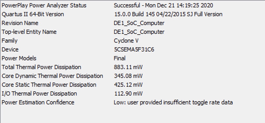

Figure 15. The power consumption output.

Appendix A: Permissions

The group approves this report for inclusion on the course website and the group also approves the video for inclusion on the course youtube channel.

Appendix B: Source code

1. Verilog: Harris corner algorithm.
2. HPS: Letter recognition and VGA drawing.
3. Matlab: Harris corner & letter recognition simulation, Import image application.
4. Database:Training pictures.
5. All the codes can be found in this Github.

Appendix C: Work distribution

All group members contributed equally to all parts of the projects. In the following table, it shows the details of the work distribution.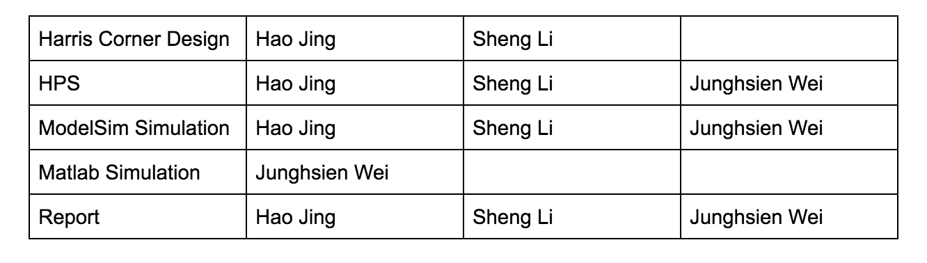

Appendix D: References

1. T. L. Chao and K. H. Wong, "An efficient FPGA implementation of the Harris corner feature detector," 2015 14th IAPR International Conference on Machine Vision Applications (MVA), Tokyo, 2015, pp. 89-93, doi: 10.1109/MVA.2015.7153140.
2. M. F. Aydogdu, M. F. Demirci and C. Kasnakoglu, "Pipelining Harris corner detection with a tiny FPGA for a mobile robot," 2013 IEEE International Conference on Robotics and Biomimetics (ROBIO), Shenzhen, 2013, pp. 2177-2184, doi: 10.1109/ROBIO.2013.6739792.
3. Gökhan Özbulak Github: https://github.com/gokhanozbulak/Harris-Detector
4. Basavarajaiah, Madhushree. “6 Basic Things to Know about Convolution.” Medium.com, Medium, 2 Apr. 2019, medium.com/@bdhuma/6-basic-things-to-know-about-convolution-daef5e1bc411.

Appendix E: Acknowledgments

We would like to thank Dr. Hunter Adams, Dr. Bruce Land, and TA Katie Bradford to give us lots of design opinions and help us debug our program. We learned the principles of Verilog, the hardware DE1-SoC memory usage, the difference between SRAM and SDRAM, and the VGA display. We really appreciate the teaching and support for the whole semester during this pandemic situation. We also want to thank our friends to help us write different letters for our system image training.

Hao Jing

M.Eng Student, 2020
Electrical and Computer Engineering
Interests: Computer Architecture, Hardware Engineering, and Digital Circuit Design
LinkedIn Profile

Sheng Li

M.Eng Student, 2020
Electrical and Computer Engineering
Interests: Machine Learning, Software Engineering, Embedded System
LinkedIn Profile

Junghsien Wei

M.Eng Student, 2020
Electrical and Computer Engineering
Interests: Robotics, Hardware Engineering, and Embedded System
LinkedIn Profile